CoProcessing

Background

This work is supported under U.S. Army Research topic A07-010 proposal number A2-3295. The name of the project is CFD Co-Processing for Unsteady Visualization, Phase II. Several factors are driving the growth of CFD simulations. Computational power of computer clusters is growing while the price of individual computers is decreasing. Distributed computing techniques allow hundreds or even thousands of computer nodes to participate in a single simulation. The benefit of this computational power is that simulations are getting more accurate and useful for predicting complex phenomena. The downside to this growth in computational power is that enormous amounts of data need to be saved and analyzed to determine the results of the simulation. The ability to generate data has outpaced our ability to save and analyze the data. This bottle neck is throttling our ability to benefit from our improved computing resources. Simulations save their states only very infrequently to minimize storage requirements. This coarse temporal sampling makes it difficult to notice some complex fluid behavior.

Research and development to address this problem has focused on various solutions including data management, data reduction and compression, saliency analysis and feature extraction. However, there are very few solutions that bring these together and introduce them in the work-flow of the researcher. Furthermore, most of these solutions focus on deploying the post-processing tools on systems that do not scale as well as the ones the simulation codes run on. As mesh size, temporal resolution, problem complexity and parameter ranges grow, the analysis and visualization world has to adapt. The visualization tool developers can no longer assume that post-processing is a serial task that happens after the simulation on a dedicated graphics workstation. Rather, the processing of the data has to be tightly integrated with the simulation in order to scale with it. This will require rethinking of many visualization algorithms, development of new ones and also creation of the next generation analysis tools that share characteristics with simulation codes and can be deployed on the same supercomputers.

Technical Objectives

The main objective of the co-processing project is to integrate core data processing with the simulation to enable scalable data analysis. We will achieve this goal by building an end-to-end co-processing system.

• Develop an Extensible and Flexible Co-Processing Library. The co-processing library developed as part of the project has to be flexible enough to be embedded in various simulation codes with relative ease. This flexibility is critical, as a library that requires a lot of effort to embed cannot be successfully deployed in a large number of simulations. The co-processing library has to be easily extensible so that users can easily deploy new analysis and visualization techniques to existing co-processing installations.

• Develop Configuration Tools for Co-Processing Configuration. Based on conversations we had with our collaborators, we concluded that it is important for the users to be able to configure the co-processor using graphical user interfaces that are part of their daily work-flow. Therefore, we will develop a

graphical user interface to setup the co-processing pipelines.

Note that all of this must be done for large data. The co-processing library will almost always be run on a distributed system. For the largest simulation, the visualization of extracts may also require a distributed system (i.e. a visualization cluster).

Build Directions

The two components for doing coprocessing are a client-side plugin and a server side library. It is recommended that they be compiled separately but from the same ParaView source revision. This is because currently the server side library uses python which due to the wrapping will try to bring in all of the paraview libraries which it could potentially need. This means that it will try to bring in objects that require a terminal window to display to which may cause problems on clusters and supercomputers.

ParaView Coprocessing Script Generator Plugin

The plugin for generating python scripts for coprocessing is a client-side plugin. The CMake option to turn on the script generator plugin is PARAVIEW_BUILD_PLUGIN_CoProcessingScriptGenerator. Note that since this is a client-side plugin that the PARAVIEW_BUILT_QT_GUI option must be on.

CoProcessing Library

The directions for building the coprocessing library can be a bit more complex. We assume that it will be built on a cluster or supercomputer. Complexities may arise from having to build mesa, use off-screen rendering, build static libraries, and/or cross-compiling. We won't go into those details here though but refer interested people to the ParaView and VTK wikis.

The addition flags that should be turned on for coprocessing include:

• BUILD_SHARED_LIBS Should normally be set to ON unless you're compiling on a machine that doesn't support shared libs (e.g. IBM BG/l).
• PARAVIEW_ENABLE_PYTHON Set to ON in order to use the scripts created from the coprocessing plugin.
• PARAVIEW_USE_MPI Set the ParaView server to use MPI to run in parallel. Also check that the proper version of MPI is getting used.
• CMAKE_BUILD_TYPE Should be set to Release in order to optimize the ParaView code.
• PARAVIEW_ENABLE_COPROCESSING The CMake option to build the coprocessing libraries.
• BUILD_COPROCESSING_ADAPTORS The CMake option to turn on code that may be useful for creating the simulation code adaptor.
• BUILD_FORTRAN_COPROCESSING_ADAPTORS The CMake option to turn on code that may be useful for creating an adaptor for a simulation code written in Fortran or C.
• PYTHON_ENABLE_MODULE_vtkCoProcessorPython On by default.
• BUILD_PYTHON_COPROCESSING_ADAPTOR Experimental code.

To test that the coprocessing library is working on your system use the command ctest -R CoProcessing. The CoProcessingTestPythonScript test does an actual coprocessing run and the CoProcessingPythonScriptGridPlot and CoProcessingPythonScriptPressurePlot test verify the output is correct. Note that by using ctest -V -R CoProcessingTestPythonScript you can see the verbose output if the test. Looking at the code for this test is a useful beginning point for learning to use the coprocessing library.

If you are using Mesa, the following options should be used:

• VTK_OPENGL_HAS_OSMESA Set to ON.
• OSMESA_INCLUDE_DIR, OPENGL_xmesa_INCLUDE_DIR and OPENGL_INCLUDE_DIR Make sure this is not set to the OpenGL version of the header files.
• OSMESA_LIBRARY, OPENGL_gl_LIBRARY and OPENGL_glu_LIBRARY Set these to the proper libraries.
• VTK_USE_OFFSCREEN Set to ON

Running the CoProcessing Script Generator

After starting the ParaView client, go to Tools->Manage Plugins, highlight CoProcessingPlugin and click Load Selected. Alternatively, if you expect to be using this plugin often you can tell ParaView to automatically load the plugin by clicking to the left of CoProcessingPlugin to expand the list and choose the Auto Load option. This will add a CoProcessing and Writers menu to the GUI.

Once the plugin is loaded, load a simulation result into ParaView that is similar to the run you wish to do coprocessing with. Normally the result will be for a discretization of the same geometry and contain the same field variables (or at least all of the field variables you wish to examine) as the simulation grid that coprocessing will be performed on. 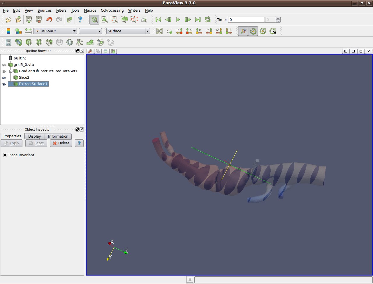The only difference between these two grids will be that the grid used for the coprocessing run will be at a much higher resolution. In the picture below, a pipeline is shown for a result from a PHASTA (REFERENCE) simulation of incompressible flow through an aortic aneurysm. The simulation results include the velocity and pressure fields and was done on a grid with 235,282 cells and 45,175 points. It is important to use the same names for the field arrays as will be used in the grids the coprocessing library will be working with. The filters specify which fields to use by their name and problems will occur if the filters cannot find the correct array. The pipeline computes the vorticity, takes 20 slices through the domain, and extracts the surface of the grid.

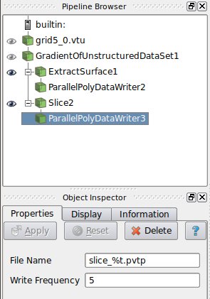
Once the pipeline is set up, you must add in the writers to use for the filters that you want results from. Do this by selecting the appropriate writer to output the results from each desired filter. In this example we create a ParallelPolyDataWriter for the Slice filter and the ExtractSurface filter. For the writer for the Slice filter we set the name of the file to be slice_%t.pvtp where %t will get replaced with the time step each time it is output. We also set the write frequency to be every fifth time step. The picture below shows this.

Similarly, we do the same for the writer for the ExtractSurface filter but we want to use a different file name and we can set a different write frequency if desired.

Note that when we hit enter we get the error message Cannot show the data in the current view although the view reported that it can show the data. This message can be ignored and is already entered as a bug to fix in ParaView.

The final step is to go through the CoProcessing->Export State wizard to associate the grid with a name that they python script uses and specify a file name for the script. The steps are:

1. Export Co-Processing State Next
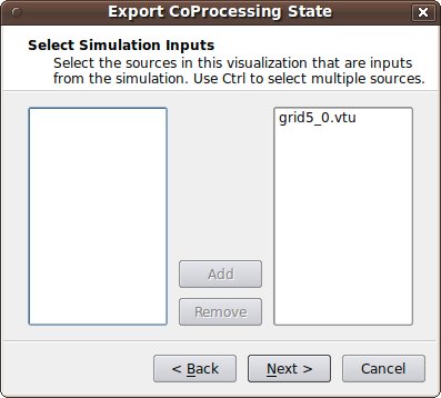
2. Select Simulation Inputs Choose which grids to use by highlighting the grid and clicking Add, then click Next.
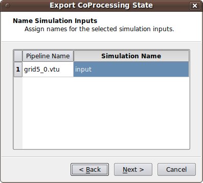
3. Name Simulation Inputs Click in the boxes under Simulation Name and change the name to what you have named the grid in your adaptor. Our convention is to use "input" for simulations with a single grid or multiblock data set.
4. Configuration We usually want the full data and not just a picture of the results so we leave "Ignore rendering components i.e. view selected and just hit Finish.
5. Save Server State: Specify the file name the script is to be save as.

The resulting python script should look something like:

<source lang="python"> try: paraview.simple except: from paraview.simple import *

cp_writers = []

def RequestDataDescription(datadescription):

   "Callback to populate the request for current timestep"
   timestep = datadescription.GetTimeStep()

   if (timestep % 5 == 0) or (timestep % 200 == 0) :
       datadescription.GetInputDescriptionByName('input').AllFieldsOn()
       datadescription.GetInputDescriptionByName('input').GenerateMeshOn()

def DoCoProcessing(datadescription):

   "Callback to do co-processing for current timestep"
   global cp_writers
   cp_writers = []
   timestep = datadescription.GetTimeStep()

   grid5_0_vtu = CreateProducer( datadescription, "input" )
   
   GradientOfUnstructuredDataSet1 = GradientOfUnstructuredDataSet( guiName="GradientOfUnstructuredDataSet1", ScalarArray=['POINTS', 'velocity'], ResultArray

Name='Vorticity', ComputeVorticity=1, FasterApproximation=0 )

   Slice2 = Slice( guiName="Slice2", SliceOffsetValues=[-10.23284210526316, -8.8684631578947375, -7.5040842105263152, -6.1397052631578966, -4.77532631578947

43, -3.4109473684210529, -2.0465684210526316, -0.68218947368421201, 0.68218947368420935, 2.0465684210526316, 3.4109473684210521, 4.7753263157894743, 6.139705 263157893, 7.5040842105263152, 8.8684631578947375, 10.23284210526316, 11.597221052631578, 12.961600000000001], SliceType="Plane" )

   SetActiveSource(GradientOfUnstructuredDataSet1)
   ExtractSurface1 = ExtractSurface( guiName="ExtractSurface1", PieceInvariant=1 )
   
   SetActiveSource(Slice2)
   ParallelPolyDataWriter3 = CreateWriter( XMLPPolyDataWriter, "slice_%t.pvtp", 5 )
   
   SetActiveSource(ExtractSurface1)
   ParallelPolyDataWriter2 = CreateWriter( XMLPPolyDataWriter, "surface_%t.pvtp", 200 )
   
   Slice2.SliceType.Origin = [-2.8049160242080688, 2.1192346811294556, 1.7417440414428711]
   Slice2.SliceType.Offset = 0.0
   Slice2.SliceType.Normal = [0.0, 0.0, 1.0]
   

   for writer in cp_writers:
       if timestep % writer.cpFrequency == 0:
           writer.FileName = writer.cpFileName.replace("%t", str(timestep))
           writer.UpdatePipeline()

def CreateProducer(datadescription, gridname):

 "Creates a producer proxy for the grid"
 if not datadescription.GetInputDescriptionByName(gridname):
   raise RuntimeError, "Simulation input name '%s' does not exist" % gridname
 grid = datadescription.GetInputDescriptionByName(gridname).GetGrid()
 producer = TrivialProducer()
 producer.GetClientSideObject().SetOutput(grid)
 producer.UpdatePipeline()
 return producer

def CreateWriter(proxy_ctor, filename, freq):

   global cp_writers
   writer = proxy_ctor()
   writer.FileName = filename
   writer.add_attribute("cpFrequency", freq)
   writer.add_attribute("cpFileName", filename)
   cp_writers.append(writer)
   return writer

</source>

Creating the Adaptor

The largest amount of work in getting coprocessing working with a simulation code is usually creating the adaptor that can pass a VTK data set or composite data set with fields specified over it. Look at the code in ParaView3/CoProcessing/CoProcessor/Testing/Cxx/PythonScriptCoProcessingExample.cxx to see how the entire coprocessing works.

Once the adaptor is created, the adaptor must be called from the simulation code in a manner similar to:

 initialize coprocessor
 for i in number of time steps
   compute fields at time step i
   call coprocessing library
     coprocessing library determines if any coprocessing needs to be performed at time step i
 finalize coprocessor