VTK/Parallel Pipeline
Introduction
VTK uses a form of parallelism called data parallelism. In this form, the data is divided amongst the processes, and each process performs the same operation on its piece of data. Advantages of data parallelism include scalability, simplified load balancing, and reduced communications overhead.
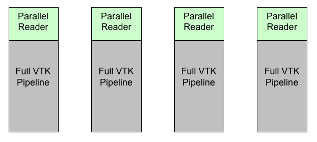
Figure 1 shows how VTK filters can be setup when running in parallel. In this example, each reader reads in a piece of the data. Usually, this can be done with very little communication between processes. Then, each reader feeds into a pipeline identical with that on the other processes. Because many of the filters in VTK use algorithms that independently process each point or cell, these filters can run in parallel with little or no communication between them. Let us see a simple example of how that works.
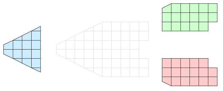
Consider the simple, 2D grid that is partitioned into three pieces shown in Figure 2. Assume that the three pieces reside on separate processes of a distributed memory computer. Because no process has global information, communications costs will be minimized if each process performs its operation only on its local information. Of course, we can only do this if the end result of the parallel operation is equivalent to the same operation on the global data.
Figure 3 demonstrates a clip filter (vtkClipDataSet for example) processing data in parallel. Each process is given the same parameters for the cut plane. The cut plane is then applied independently on each piece of the data. When the pieces are brought back together, we see that the result is the entire data set properly cut by the plane.
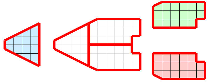
Not all visualization algorithms can operate on pieces without information on neighboring cells. Consider the operation of extracting external faces as shown in Figure 4. The external face operation identifies all faces that have no local neighbors. When we bring the pieces together, we see that some internal faces have been incorrectly identified as being external. These false positives on the faces occur whenever two neighboring cells are placed in separate processes.
The external face operation in our example fails because some important global information is missing from the local processing. The processes need some data that is not local to them, but they do not need all the data. They only need to know about cells in other partitions that are neighbors to the local cells.
We can solve this local/global problem with the introduction of ghost cells. Ghost cells are cells that belong to one partition of the data and are duplicated on other partitions. The introduction of ghost cells is performed through neighborhood information and organized in levels. For a given partition, any cell neighboring a cell in the partition but not belonging to the partition itself is a ghost cell 1. Any cell neighboring a ghost cell at level 1 that does not belong to level 1 or the original partition is at level 2. Further levels are defined recursively. We define ghost cells in this way because it provides a simple distance metric to the cells of a partition and allows filters to easily specify the minimal or near minimal set of ghost cells required for proper operation.
Let us apply the use of ghost cells to our example of extracting external faces. Figure 5 shows the same partitions with a layer of ghost cells added. When the external face algorithm is run again, some faces are still inappropriately classified as external. However, all of these faces are attached to ghost cells. These ghost faces are easily culled, and the end result is the appropriate external faces.


