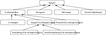
Figure 5.1: Sample class inheritance diagram.
This chapter introduces the statistics functionalities in Insight. The statistics subsystem’s primary purpose is to provide general capabilities for statistical pattern classification. However, its use is not limited for classification. Users might want to use data containers and algorithms in the statistics subsystem to perform other statistical analysis or to preprocess image data for other tasks.
The statistics subsystem mainly consists of three parts: data container classes, statistical algorithms, and the classification framework. In this chapter, we will discuss each major part in that order.
An itk::Statistics::Sample object is a data container of elements that we call measurement vectors. A measurement vector is an array of values (of the same type) measured on an object (In images, it can be a vector of the gray intensity value and/or the gradient value of a pixel). Strictly speaking from the design of the Sample class, a measurement vector can be any class derived from itk::FixedArray, including FixedArray itself.
The source code for this section can be found in the file
ListSample.cxx.
This example illustrates the common interface of the Sample class in Insight.
Different subclasses of itk::Statistics::Sample expect different sets of template arguments. In this example, we use the itk::Statistics::ListSample class that requires the type of measurement vectors. The ListSample uses STL vector to store measurement vectors. This class conforms to the common interface of Sample. Most methods of the Sample class interface are for retrieving measurement vectors, the size of a container, and the total frequency. In this example, we will see those information retrieving methods in addition to methods specific to the ListSample class for data input.
To use the ListSample class, we include the header file for the class.
We need another header for measurement vectors. We are going to use the itk::Vector class which is a subclass of the itk::FixedArray class.
The following code snippet defines the measurement vector type as a three component float itk::Vector. The MeasurementVectorType is the measurement vector type in the SampleType. An object is instantiated at the third line.
In the above code snippet, the namespace specifier for ListSample is itk::Statistics:: instead of the usual namespace specifier for other ITK classes, itk::.
The newly instantiated object does not have any data in it. We have two different ways of storing data elements. The first method is using the PushBack method.
The previous code increases the size of the container by one and stores mv as the first data element in it.
The other way to store data elements is calling the Resize method and then calling the SetMeasurementVector() method with a measurement vector. The following code snippet increases the size of the container to three and stores two measurement vectors at the second and the third slot. The measurement vector stored using the PushBack method above is still at the first slot.
We have seen how to create an ListSample object and store measurement vectors using the ListSample-specific interface. The following code shows the common interface of the Sample class. The Size method returns the number of measurement vectors in the sample. The primary data stored in Sample subclasses are measurement vectors. However, each measurement vector has its associated frequency of occurrence within the sample. For the ListSample and the adaptor classes (see Section 5.1.2), the frequency value is always one. itk::Statistics::Histogram can have a varying frequency (float type) for each measurement vector. We retrieve measurement vectors using the GetMeasurementVector(unsigned long instance identifier), and frequency using the GetFrequency(unsigned long instance identifier).
The output should look like the following:
id = 0 measurement vector = 1 2 4 frequency = 1
id = 1 measurement vector = 2 4 5 frequency = 1
id = 2 measurement vector = 3 8 6 frequency = 1
We can get the same result with its iterator.
The last method defined in the Sample class is the GetTotalFrequency() method that returns the sum of frequency values associated with every measurement vector in a container. In the case of ListSample and the adaptor classes, the return value should be exactly the same as that of the Size() method, because the frequency values are always one for each measurement vector. However, for the itk::Statistics::Histogram, the frequency values can vary. Therefore, if we want to develop a general algorithm to calculate the sample mean, we must use the GetTotalFrequency() method instead of the Size() method.
There are two adaptor classes that provide the common itk::Statistics::Sample interfaces for itk::Image and itk::PointSet, two fundamental data container classes found in ITK. The adaptor classes do not store any real data elements themselves. These data come from the source data container plugged into them. First, we will describe how to create an itk::Statistics::ImageToListSampleAdaptor and then an itk::Statistics::PointSetToListSampleAdaptor object.
The source code for this section can be found in the file
ImageToListSampleAdaptor.cxx.
This example shows how to instantiate an itk::Statistics::ImageToListSampleAdaptor object and plug-in an itk::Image object as the data source for the adaptor.
In this example, we use the ImageToListSampleAdaptor class that requires the input type of Image as the template argument. To users of the ImageToListSampleAdaptor, the pixels of the input image are treated as measurement vectors. The ImageToListSampleAdaptor is one of two adaptor classes among the subclasses of the itk::Statistics::Sample. That means an ImageToListSampleAdaptor object does not store any real data. The data comes from other ITK data container classes. In this case, an instance of the Image class is the source of the data.
To use an ImageToListSampleAdaptor object, include the header file for the class. Since we are using an adaptor, we also should include the header file for the Image class. For illustration, we use the itk::RandomImageSource that generates an image with random pixel values. So, we need to include the header file for this class. Another convenient filter is the itk::ComposeImageFilter which creates an image with pixels of array type from one or more input images composed of pixels of scalar type. Since an element of a Sample object is a measurement vector, you cannot plug in an image of scalar pixels. However, if we want to use an image of scalar pixels without the help from the ComposeImageFilter, we can use the itk::Statistics::ScalarImageToListSampleAdaptor class that is derived from the itk::Statistics::ImageToListSampleAdaptor. The usage of the ScalarImageToListSampleAdaptor is identical to that of the ImageToListSampleAdaptor.
We assume you already know how to create an image. The following code snippet will create a 2D image of float pixels filled with random values.
using FloatImage2DType = itk::Image<float,2>;
itk::RandomImageSource<FloatImage2DType>::Pointer random;
random = itk::RandomImageSource<FloatImage2DType>::New();
random->SetMin( 0.0 );
random->SetMax( 1000.0 );
using SpacingValueType = FloatImage2DType::SpacingValueType;
using SizeValueType = FloatImage2DType::SizeValueType;
using PointValueType = FloatImage2DType::PointValueType;
SizeValueType size[2] = {20, 20};
random->SetSize( size );
SpacingValueType spacing[2] = {0.7, 2.1};
random->SetSpacing( spacing );
PointValueType origin[2] = {15, 400};
random->SetOrigin( origin );
We now have an instance of Image and need to cast it to an Image object with an array pixel type (anything derived from the itk::FixedArray class such as itk::Vector, itk::Point, itk::RGBPixel, or itk::CovariantVector).
Since the image pixel type is float in this example, we will use a single element float FixedArray as our measurement vector type. And that will also be our pixel type for the cast filter.
using MeasurementVectorType = itk::FixedArray< float, 1 >;
using ArrayImageType = itk::Image< MeasurementVectorType, 2 >;
using CasterType =
itk::ComposeImageFilter< FloatImage2DType, ArrayImageType >;
CasterType::Pointer caster = CasterType::New();
caster->SetInput( random->GetOutput() );
caster->Update();
Up to now, we have spent most of our time creating an image suitable for the adaptor. Actually, the hard part of this example is done. Now, we just define an adaptor with the image type and instantiate an object.
The final task is to plug in the image object to the adaptor. After that, we can use the common methods and iterator interfaces shown in Section 5.1.1.
If we are interested only in pixel values, the ScalarImageToListSampleAdaptor (scalar pixels) or the ImageToListSampleAdaptor (vector pixels) would be sufficient. However, if we want to perform some statistical analysis on spatial information (image index or pixel’s physical location) and pixel values altogether, we want to have a measurement vector that consists of a pixel’s value and physical position. In that case, we can use the itk::Statistics::JointDomainImageToListSampleAdaptor class. With this class, when we call the GetMeasurementVector() method, the returned measurement vector is composed of the physical coordinates and pixel values. The usage is almost the same as with ImageToListSampleAdaptor. One important difference between JointDomainImageToListSampleAdaptor and the other two image adaptors is that the JointDomainImageToListSampleAdaptor has the SetNormalizationFactors() method. Each component of a measurement vector from the JointDomainImageToListSampleAdaptor is divided by the corresponding component value from the supplied normalization factors.
The source code for this section can be found in the file
PointSetToListSampleAdaptor.cxx.
We will describe how to use itk::PointSet as a itk::Statistics::Sample using an adaptor in this example.
The itk::Statistics::PointSetToListSampleAdaptor class requires a PointSet as input. The PointSet class is an associative data container. Each point in a PointSet object can have an associated optional data value. For the statistics subsystem, the current implementation of PointSetToListSampleAdaptor takes only the point part into consideration. In other words, the measurement vectors from a PointSetToListSampleAdaptor object are points from the PointSet object that is plugged into the adaptor object.
To use an PointSetToListSampleAdaptor class, we include the header file for the class.
Since we are using an adaptor, we also include the header file for the PointSet class.
Next we create a PointSet object. The following code snippet will create a PointSet object that stores points (its coordinate value type is float) in 3D space.
Note that the short type used in the declaration of PointSetType pertains to the pixel type associated with every point, not to the type used to represent point coordinates. If we want to change the type of the point in terms of the coordinate value and/or dimension, we have to modify the TMeshTraits (one of the optional template arguments for the PointSet class). The easiest way of creating a custom mesh traits instance is to specialize the existing itk::DefaultStaticMeshTraits. By specifying the TCoordRep template argument, we can change the coordinate value type of a point. By specifying the VPointDimension template argument, we can change the dimension of the point. As mentioned earlier, a PointSetToListSampleAdaptor object cares only about the points, and the type of measurement vectors is the type of points.
To make the example a little bit realistic, we add two points into the pointSet.
Now we have a PointSet object with two points in it. The PointSet is ready to be plugged into the adaptor. First, we create an instance of the PointSetToListSampleAdaptor class with the type of the input PointSet object.
Second, all we have to do is plug in the PointSet object to the adaptor. After that, we can use the common methods and iterator interfaces shown in Section 5.1.1.
The source code for this section can be found in the file
PointSetToAdaptor.cxx.
We will describe how to use itk::PointSet as a Sample using an adaptor in this example.
itk::Statistics::PointSetToListSampleAdaptor class requires the type of input itk::PointSet object. The itk::PointSet class is an associative data container. Each point in a PointSet object can have its associated data value (optional). For the statistics subsystem, current implementation of PointSetToListSampleAdaptor takes only the point part into consideration. In other words, the measurement vectors from a PointSetToListSampleAdaptor object are points from the PointSet object that is plugged-into the adaptor object.
To use, an itk::PointSetToListSampleAdaptor object, we include the header file for the class.
Since, we are using an adaptor, we also include the header file for the itk::PointSet class.
We assume you already know how to create an itk::PointSet object. The following code snippet will create a 2D image of float pixels filled with random values.
using FloatPointSet2DType = itk::PointSet<float,2>;
itk::RandomPointSetSource<FloatPointSet2DType>::Pointer random;
random = itk::RandomPointSetSource<FloatPointSet2DType>::New();
random->SetMin(0.0);
random->SetMax(1000.0);
unsigned long size[2] = {20, 20};
random->SetSize(size);
float spacing[2] = {0.7, 2.1};
random->SetSpacing( spacing );
float origin[2] = {15, 400};
random->SetOrigin( origin );
We now have an itk::PointSet object and need to cast it to an itk::PointSet object with array type (anything derived from the itk::FixedArray class) pixels.
Since, the itk::PointSet object’s pixel type is float, We will use single element float itk::FixedArray as our measurement vector type. And that will also be our pixel type for the cast filter.
using MeasurementVectorType = itk::FixedArray< float, 1 >;
using ArrayPointSetType = itk::PointSet< MeasurementVectorType, 2 >;
using CasterType = itk::ScalarToArrayCastPointSetFilter< FloatPointSet2DType,
ArrayPointSetType >;
CasterType::Pointer caster = CasterType::New();
caster->SetInput( random->GetOutput() );
caster->Update();
Up to now, we spend most of time to prepare an itk::PointSet object suitable for the adaptor. Actually, the hard part of this example is done. Now, we must define an adaptor with the image type and instantiate an object.
The final thing we have to is to plug-in the image object to the adaptor. After that, we can use the common methods and iterator interfaces shown in 5.1.1.
The source code for this section can be found in the file
Histogram.cxx.
This example shows how to create an itk::Statistics::Histogram object and use it.
We call an instance in a Histogram object a bin. The Histogram differs from the itk::Statistics::ListSample, itk::Statistics::ImageToListSampleAdaptor, or itk::Statistics::PointSetToListSampleAdaptor in significant ways. Histograms can have a variable number of values (float type) for each measurement vector, while the three other classes have a fixed value (one) for all measurement vectors. Also those array-type containers can have multiple instances (data elements) with identical measurement vector values. However, in a Histogram object, there is one unique instance for any given measurement vector.
Here we create a histogram with dense frequency containers. In this example we will not have any zero-frequency measurements, so the dense frequency container is the appropriate choice. If the histogram is expected to have many empty (zero) bins, a sparse frequency container would be the better option. Here we also set the size of the measurement vectors to be 2 components.
using MeasurementType = float;
using FrequencyContainerType = itk::Statistics::DenseFrequencyContainer2;
using FrequencyType = FrequencyContainerType::AbsoluteFrequencyType;
constexpr unsigned int numberOfComponents = 2;
using HistogramType = itk::Statistics::Histogram< MeasurementType,
FrequencyContainerType >;
HistogramType::Pointer histogram = HistogramType::New();
histogram->SetMeasurementVectorSize( numberOfComponents );
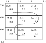
We initialize it as a 3×3 histogram with equal size intervals.
HistogramType::SizeType size( numberOfComponents );
size.Fill(3);
HistogramType::MeasurementVectorType lowerBound( numberOfComponents );
HistogramType::MeasurementVectorType upperBound( numberOfComponents );
lowerBound[0] = 1.1;
lowerBound[1] = 2.6;
upperBound[0] = 7.1;
upperBound[1] = 8.6;
histogram->Initialize(size, lowerBound, upperBound );
Now the histogram is ready for storing frequency values. We will fill each bin’s frequency according to the Figure 5.2. There are three ways of accessing data elements in the histogram:
In this example, the index (0,0) refers the same bin as the instance identifier (0) refers to. The instance identifier of the index (0, 1) is (3), (0, 2) is (6), (2, 2) is (8), and so on.
histogram->SetFrequency(0UL, static_cast<FrequencyType>(0.0));
histogram->SetFrequency(1UL, static_cast<FrequencyType>(2.0));
histogram->SetFrequency(2UL, static_cast<FrequencyType>(3.0));
histogram->SetFrequency(3UL, static_cast<FrequencyType>(2.0f));
histogram->SetFrequency(4UL, static_cast<FrequencyType>(0.5f));
histogram->SetFrequency(5UL, static_cast<FrequencyType>(1.0f));
histogram->SetFrequency(6UL, static_cast<FrequencyType>(5.0f));
histogram->SetFrequency(7UL, static_cast<FrequencyType>(2.5f));
histogram->SetFrequency(8UL, static_cast<FrequencyType>(0.0f));
Let us examine if the frequency is set correctly by calling the GetFrequency(index) method. We can use the GetFrequency(instance identifier) method for the same purpose.
For test purposes, we create a measurement vector and an index that belongs to the center bin.
We retrieve the measurement vector at the index value (1, 1), the center bin’s measurement vector. The output is [4.1, 5.6].
Since all the measurement vectors are unique in the Histogram class, we can determine the index from a measurement vector.
In a similar way, we can get the instance identifier from the index.
If we want to check if an index is valid, we use the method IsIndexOutOfBounds(index). The following code snippet fills the index variable with (100, 100). It is obviously not a valid index.
The following code snippets show how to get the histogram size and frequency dimension.
The Histogram class has a quantile calculation method, Quantile(dimension, percent). The following code returns the 50th percentile along the first dimension. Note that the quantile calculation considers only one dimension.
The source code for this section can be found in the file
Subsample.cxx.
The itk::Statistics::Subsample is a derived sample. In other words, it requires another itk::Statistics::Sample object for storing measurement vectors. The Subsample class stores a subset of instance identifiers from another Sample object. Any Sample’s subclass can be the source Sample object. You can create a Subsample object out of another Subsample object. The Subsample class is useful for storing classification results from a test Sample object or for just extracting some part of interest in a Sample object. Another good use of Subsample is sorting a Sample object. When we use an itk::Image object as the data source, we do not want to change the order of data elements in the image. However, we sometimes want to sort or select data elements according to their order. Statistics algorithms for this purpose accepts only Subsample objects as inputs. Changing the order in a Subsample object does not change the order of the source sample.
To use a Subsample object, we include the header files for the class itself and a Sample class. We will use the itk::Statistics::ListSample as the input sample.
We need another header for measurement vectors. We are going to use the itk::Vector class in this example.
The following code snippet will create a ListSample object with three-component float measurement vectors and put three measurement vectors into the list.
using MeasurementVectorType = itk::Vector< float, 3 >;
using SampleType = itk::Statistics::ListSample< MeasurementVectorType >;
SampleType::Pointer sample = SampleType::New();
MeasurementVectorType mv;
mv[0] = 1.0;
mv[1] = 2.0;
mv[2] = 4.0;
sample->PushBack(mv);
mv[0] = 2.0;
mv[1] = 4.0;
mv[2] = 5.0;
sample->PushBack(mv);
mv[0] = 3.0;
mv[1] = 8.0;
mv[2] = 6.0;
sample->PushBack(mv);
To create a Subsample instance, we define the type of the Subsample with the source sample type, in this case, the previously defined SampleType. As usual, after that, we call the New() method to create an instance. We must plug in the source sample, sample, using the SetSample() method. However, with regard to data elements, the Subsample is empty. We specify which data elements, among the data elements in the Sample object, are part of the Subsample. There are two ways of doing that. First, if we want to include every data element (instance) from the sample, we simply call the InitializeWithAllInstances() method like the following:
This method is useful when we want to create a Subsample object for sorting all the data elements in a Sample object. However, in most cases, we want to include only a subset of a Sample object. For this purpose, we use the AddInstance(instance identifier) method in this example. In the following code snippet, we include only the first and last instance in our subsample object from the three instances of the Sample class.
The Subsample is ready for use. The following code snippet shows how to use Iterator interfaces.
As mentioned earlier, the instances in a Subsample can be sorted without changing the order in the source Sample. For this purpose, the Subsample provides an additional instance indexing scheme. The indexing scheme is just like the instance identifiers for the Sample. The index is an integer value starting at 0, and the last value is one less than the number of all instances in a Subsample. The Swap(0, 1) method, for example, swaps two instance identifiers of the first data element and the second element in the Subsample. Internally, the Swap() method changes the instance identifiers in the first and second position. Using indices, we can print out the effects of the Swap() method. We use the GetMeasurementVectorByIndex(index) to get the measurement vector at the index position. However, if we want to use the common methods of Sample that accepts instance identifiers, we call them after we get the instance identifiers using GetInstanceIdentifier(index) method.
Since we are using a ListSample object as the source sample, the following code snippet will return the same value (2) for the Size() and the GetTotalFrequency() methods. However, if we used a Histogram object as the source sample, the two return values might be different because a Histogram allows varying frequency values for each instance.
If we want to remove all instances that are associated with the Subsample, we call the Clear() method. After this invocation, the Size() and the GetTotalFrequency() methods return 0.
The source code for this section can be found in the file
MembershipSample.cxx.
The itk::Statistics::MembershipSample is derived from the class itk::Statistics::Sample that associates a class label with each measurement vector. It needs another Sample object for storing measurement vectors. A MembershipSample object stores a subset of instance identifiers from another Sample object. Any subclass of Sample can be the source Sample object. The MembershipSample class is useful for storing classification results from a test Sample object. The MembershipSample class can be considered as an associative container that stores measurement vectors, frequency values, and class labels.
To use a MembershipSample object, we include the header files for the class itself and the Sample class. We will use the itk::Statistics::ListSample as the input sample. We need another header for measurement vectors. We are going to use the itk::Vector class which is a subclass of the itk::FixedArray.
The following code snippet will create a ListSample object with three-component float measurement vectors and put three measurement vectors in the ListSample object.
using MeasurementVectorType = itk::Vector< float, 3 >;
using SampleType = itk::Statistics::ListSample< MeasurementVectorType >;
SampleType::Pointer sample = SampleType::New();
MeasurementVectorType mv;
mv[0] = 1.0;
mv[1] = 2.0;
mv[2] = 4.0;
sample->PushBack(mv);
mv[0] = 2.0;
mv[1] = 4.0;
mv[2] = 5.0;
sample->PushBack(mv);
mv[0] = 3.0;
mv[1] = 8.0;
mv[2] = 6.0;
sample->PushBack(mv);
To create a MembershipSample instance, we define the type of the MembershipSample using the source sample type using the previously defined SampleType. As usual, after that, we call the New() method to create an instance. We must plug in the source sample, Sample, using the SetSample() method. We provide class labels for data instances in the Sample object using the AddInstance() method. As the required initialization step for the membershipSample, we must call the SetNumberOfClasses() method with the number of classes. We must add all instances in the source sample with their class labels. In the following code snippet, we set the first instance’ class label to 0, the second to 0, the third (last) to 1. After this, the membershipSample has two Subsample objects. And the class labels for these two Subsample objects are 0 and 1. The 0 class Subsample object includes the first and second instances, and the 1 class includes the third instance.
using MembershipSampleType = itk::Statistics::MembershipSample<SampleType>;
MembershipSampleType::Pointer membershipSample =
MembershipSampleType::New();
membershipSample->SetSample(sample);
membershipSample->SetNumberOfClasses(2);
membershipSample->AddInstance(0U, 0UL );
membershipSample->AddInstance(0U, 1UL );
membershipSample->AddInstance(1U, 2UL );
The Size() and GetTotalFrequency() returns the same information that Sample does.
The membershipSample is ready for use. The following code snippet shows how to use the Iterator interface. The MembershipSample’s Iterator has an additional method that returns the class label (GetClassLabel()).
MembershipSampleType::ConstIterator iter = membershipSample->Begin();
while ( iter != membershipSample->End() )
{
std::cout << "instance identifier = " << iter.GetInstanceIdentifier()
<< "\t measurement vector = "
<< iter.GetMeasurementVector()
<< "\t frequency = "
<< iter.GetFrequency()
<< "\t class label = "
<< iter.GetClassLabel()
<< std::endl;
++iter;
}
To see the numbers of instances in each class subsample, we use the Size() method of the ClassSampleType instance returned by the GetClassSample(index) method.
We call the GetClassSample() method to get the class subsample in the membershipSample. The MembershipSampleType::ClassSampleType is actually a specialization of the itk::Statistics::Subsample. We print out the instance identifiers, measurement vectors, and frequency values that are part of the class. The output will be two lines for the two instances that belong to the class 0.
MembershipSampleType::ClassSampleType::ConstPointer classSample =
membershipSample->GetClassSample( 0 );
MembershipSampleType::ClassSampleType::ConstIterator c_iter =
classSample->Begin();
while ( c_iter != classSample->End() )
{
std::cout << "instance identifier = " << c_iter.GetInstanceIdentifier()
<< "\t measurement vector = "
<< c_iter.GetMeasurementVector()
<< "\t frequency = "
<< c_iter.GetFrequency() << std::endl;
++c_iter;
}
The source code for this section can be found in the file
MembershipSampleGenerator.cxx.
To use, an MembershipSample object, we include the header files for the class itself and a Sample class. We will use the ListSample as the input sample.
We need another header for measurement vectors. We are going to use the itk::Vector class which is a subclass of the itk::FixedArray in this example.
The following code snippet will create a ListSample object with three-component float measurement vectors and put three measurement vectors in the ListSample object.
using MeasurementVectorType = itk::Vector< float, 3 >;
using SampleType = itk::Statistics::ListSample< MeasurementVectorType >;
SampleType::Pointer sample = SampleType::New();
MeasurementVectorType mv;
mv[0] = 1.0;
mv[1] = 2.0;
mv[2] = 4.0;
sample->PushBack(mv);
mv[0] = 2.0;
mv[1] = 4.0;
mv[2] = 5.0;
sample->PushBack(mv);
mv[0] = 3.0;
mv[1] = 8.0;
mv[2] = 6.0;
sample->PushBack(mv);
To create a MembershipSample instance, we define the type of the MembershipSample with the source sample type, in this case, previously defined SampleType. As usual, after that, we call New() method to instantiate an instance. We must plug in the source sample, sample object using the SetSample(source sample) method. However, in regard to class labels, the membershipSample is empty. We provide class labels for data instances in the sample object using the AddInstance(class label, instance identifier) method. As the required initialization step for the membershipSample, we must call the SetNumberOfClasses(number of classes) method with the number of classes. We must add all instances in the source sample with their class labels. In the following code snippet, we set the first instance class label to 0, the second to 0, the third (last) to 1. After this, the membershipSample has two Subclass objects. And the class labels for these two Subclass are 0 and 1. The 0 class Subsample object includes the first and second instances, and the 1 class includes the third instance.
using MembershipSampleType =
itk::Statistics::MembershipSample< SampleType >;
MembershipSampleType::Pointer membershipSample =
MembershipSampleType::New();
membershipSample->SetSample(sample);
membershipSample->SetNumberOfClasses(2);
membershipSample->AddInstance(0U, 0UL );
membershipSample->AddInstance(0U, 1UL );
membershipSample->AddInstance(1U, 2UL );
The Size() and GetTotalFrequency() methods return the same values as the sample.
The membershipSample is ready for use. The following code snippet shows how to use Iterator interfaces. The MembershipSampleIterator has an additional method that returns the class label (GetClassLabel()).
MembershipSampleType::Iterator iter = membershipSample->Begin();
while ( iter != membershipSample->End() )
{
std::cout << "instance identifier = " << iter.GetInstanceIdentifier()
<< "\t measurement vector = "
<< iter.GetMeasurementVector()
<< "\t frequency = "
<< iter.GetFrequency()
<< "\t class label = "
<< iter.GetClassLabel()
<< std::endl;
++iter;
}
To see the numbers of instances in each class subsample, we use the GetClassSampleSize(class label) method.
We call the GetClassSample(class label) method to get the class subsample in the membershipSample. The MembershipSampleType::ClassSampleType is actually an specialization of the itk::Statistics::Subsample. We print out the instance identifiers, measurement vectors, and frequency values that are part of the class. The output will be two lines for the two instances that belong to the class 0.
MembershipSampleType::ClassSampleType::Pointer classSample =
membershipSample->GetClassSample(0);
MembershipSampleType::ClassSampleType::Iterator c_iter =
classSample->Begin();
while ( c_iter != classSample->End() )
{
std::cout << "instance identifier = " << c_iter.GetInstanceIdentifier()
<< "\t measurement vector = "
<< c_iter.GetMeasurementVector()
<< "\t frequency = "
<< c_iter.GetFrequency() << std::endl;
++c_iter;
}
The source code for this section can be found in the file
KdTree.cxx.
The itk::Statistics::KdTree implements a data structure that separates samples in a k-dimension space. The std::vector class is used here as the container for the measurement vectors from a sample.
We define the measurement vector type and instantiate a itk::Statistics::ListSample object, and then put 1000 measurement vectors in the object.
using MeasurementVectorType = itk::Vector< float, 2 >;
using SampleType = itk::Statistics::ListSample< MeasurementVectorType >;
SampleType::Pointer sample = SampleType::New();
sample->SetMeasurementVectorSize( 2 );
MeasurementVectorType mv;
for (unsigned int i = 0; i < 1000; ++i )
{
mv[0] = (float) i;
mv[1] = (float) ((1000 - i) / 2 );
sample->PushBack( mv );
}
The following code snippet shows how to create two KdTree objects. The first object itk::Statistics::KdTreeGenerator has a minimal set of information (partition dimension, partition value, and pointers to the left and right child nodes). The second tree from the itk::Statistics::WeightedCentroidKdTreeGenerator has additional information such as the number of children under each node, and the vector sum of the measurement vectors belonging to children of a particular node. WeightedCentroidKdTreeGenerator and the resulting k-d tree structure were implemented based on the description given in the paper by Kanungo et al [28].
The instantiation and input variables are exactly the same for both tree generators. Using the SetSample() method we plug-in the source sample. The bucket size input specifies the limit on the maximum number of measurement vectors that can be stored in a terminal (leaf) node. A bigger bucket size results in a smaller number of nodes in a tree. It also affects the efficiency of search. With many small leaf nodes, we might experience slower search performance because of excessive boundary comparisons.
using TreeGeneratorType = itk::Statistics::KdTreeGenerator< SampleType >;
TreeGeneratorType::Pointer treeGenerator = TreeGeneratorType::New();
treeGenerator->SetSample( sample );
treeGenerator->SetBucketSize( 16 );
treeGenerator->Update();
using CentroidTreeGeneratorType =
itk::Statistics::WeightedCentroidKdTreeGenerator<SampleType>;
CentroidTreeGeneratorType::Pointer centroidTreeGenerator =
CentroidTreeGeneratorType::New();
centroidTreeGenerator->SetSample( sample );
centroidTreeGenerator->SetBucketSize( 16 );
centroidTreeGenerator->Update();
After the generation step, we can get the pointer to the kd-tree from the generator by calling the GetOutput() method. To traverse a kd-tree, we have to use the GetRoot() method. The method will return the root node of the tree. Every node in a tree can have its left and/or right child node. To get the child node, we call the Left() or the Right() method of a node (these methods do not belong to the kd-tree but to the nodes).
We can get other information about a node by calling the methods described below in addition to the child node pointers.
using TreeType = TreeGeneratorType::KdTreeType;
using NodeType = TreeType::KdTreeNodeType;
TreeType::Pointer tree = treeGenerator->GetOutput();
TreeType::Pointer centroidTree = centroidTreeGenerator->GetOutput();
NodeType⋆ root = tree->GetRoot();
if ( root->IsTerminal() )
{
std::cout << "Root node is a terminal node." << std::endl;
}
else
{
std::cout << "Root node is not a terminal node." << std::endl;
}
unsigned int partitionDimension;
float partitionValue;
root->GetParameters( partitionDimension, partitionValue);
std::cout << "Dimension chosen to split the space = "
<< partitionDimension << std::endl;
std::cout << "Split point on the partition dimension = "
<< partitionValue << std::endl;
std::cout << "Address of the left chile of the root node = "
<< root->Left() << std::endl;
std::cout << "Address of the right chile of the root node = "
<< root->Right() << std::endl;
root = centroidTree->GetRoot();
std::cout << "Number of the measurement vectors under the root node"
<< " in the tree hierarchy = " << root->Size() << std::endl;
NodeType::CentroidType centroid;
root->GetWeightedCentroid( centroid );
std::cout << "Sum of the measurement vectors under the root node = "
<< centroid << std::endl;
std::cout << "Number of the measurement vectors under the left child"
<< " of the root node = " << root->Left()->Size() << std::endl;
In the following code snippet, we query the three nearest neighbors of the queryPoint on the two tree. The results and procedures are exactly the same for both. First we define the point from which distances will be measured.
Then we instantiate the type of a distance metric, create an object of this type and set the origin of coordinates for measuring distances. The GetMeasurementVectorSize() method returns the length of each measurement vector stored in the sample.
using DistanceMetricType =
itk::Statistics::EuclideanDistanceMetric<MeasurementVectorType>;
DistanceMetricType::Pointer distanceMetric = DistanceMetricType::New();
DistanceMetricType::OriginType origin( 2 );
for ( unsigned int i = 0; i < sample->GetMeasurementVectorSize(); ++i )
{
origin[i] = queryPoint[i];
}
distanceMetric->SetOrigin( origin );
We can now set the number of neighbors to be located and the point coordinates to be used as a reference system.
unsigned int numberOfNeighbors = 3;
TreeType::InstanceIdentifierVectorType neighbors;
tree->Search( queryPoint, numberOfNeighbors, neighbors);
std::cout <<
"\n⋆⋆⋆ kd-tree knn search result using an Euclidean distance metric:"
<< std::endl
<< "query point = [" << queryPoint << "]" << std::endl
<< "k = " << numberOfNeighbors << std::endl;
std::cout << "measurement vector : distance from querry point " << std::endl;
std::vector<double> distances1 (numberOfNeighbors);
for ( unsigned int i = 0; i < numberOfNeighbors; ++i )
{
distances1[i] = distanceMetric->Evaluate(
tree->GetMeasurementVector( neighbors[i] ));
std::cout << "[" << tree->GetMeasurementVector( neighbors[i] )
<< "] : "
<< distances1[i]
<< std::endl;
}
Instead of using an Euclidean distance metric, Tree itself can also return the distance vector. Here we get the distance values from tree and compare them with previous values.
std::vector<double> distances2;
tree->Search( queryPoint, numberOfNeighbors, neighbors, distances2 );
std::cout << "\n⋆⋆⋆ kd-tree knn search result directly from tree:"
<< std::endl
<< "query point = [" << queryPoint << "]" << std::endl
<< "k = " << numberOfNeighbors << std::endl;
std::cout << "measurement vector : distance from querry point " << std::endl;
for ( unsigned int i = 0; i < numberOfNeighbors; ++i )
{
std::cout << "[" << tree->GetMeasurementVector( neighbors[i] )
<< "] : "
<< distances2[i]
<< std::endl;
if ( itk::Math::NotAlmostEquals( distances2[i], distances1[i] ) )
{
std::cerr << "Mismatched distance values by tree." << std::endl;
return EXIT_FAILURE;
}
}
As previously indicated, the interface for finding nearest neighbors in the centroid tree is very similar.
std::vector<double> distances3;
centroidTree->Search(
queryPoint, numberOfNeighbors, neighbors, distances3 );
centroidTree->Search( queryPoint, numberOfNeighbors, neighbors );
std::cout << "\n⋆⋆⋆ Weighted centroid kd-tree knn search result:"
<< std::endl
<< "query point = [" << queryPoint << "]" << std::endl
<< "k = " << numberOfNeighbors << std::endl;
std::cout << "measurement vector : distance_by_distMetric : distance_by_tree"
<< std::endl;
std::vector<double> distances4 (numberOfNeighbors);
for ( unsigned int i = 0; i < numberOfNeighbors; ++i )
{
distances4[i] = distanceMetric->Evaluate(
centroidTree->GetMeasurementVector( neighbors[i]));
std::cout << "[" << centroidTree->GetMeasurementVector( neighbors[i] )
<< "] : "
<< distances4[i]
<< " : "
<< distances3[i]
<< std::endl;
if ( itk::Math::NotAlmostEquals( distances2[i], distances1[i] ) )
{
std::cerr << "Mismatched distance values by centroid tree." << std::endl;
return EXIT_FAILURE;
}
}
KdTree also supports searching points within a hyper-spherical kernel. We specify the radius and call the Search() method. In the case of the KdTree, this is done with the following lines of code.
double radius = 437.0;
tree->Search( queryPoint, radius, neighbors );
std::cout << "\nSearching points within a hyper-spherical kernel:"
<< std::endl;
std::cout << "⋆⋆⋆ kd-tree radius search result:" << std::endl
<< "query point = [" << queryPoint << "]" << std::endl
<< "search radius = " << radius << std::endl;
std::cout << "measurement vector : distance" << std::endl;
for ( auto neighbor : neighbors)
{
std::cout << "[" << tree->GetMeasurementVector( neighbor )
<< "] : "
<< distanceMetric->Evaluate(
tree->GetMeasurementVector( neighbor))
<< std::endl;
}
In the case of the centroid KdTree, the Search() method is used as illustrated by the following code.
centroidTree->Search( queryPoint, radius, neighbors );
std::cout << "\n⋆⋆⋆ Weighted centroid kd-tree radius search result:"
<< std::endl
<< "query point = [" << queryPoint << "]" << std::endl
<< "search radius = " << radius << std::endl;
std::cout << "measurement vector : distance" << std::endl;
for ( auto neighbor : neighbors)
{
std::cout << "[" << centroidTree->GetMeasurementVector( neighbor )
<< "] : "
<< distanceMetric->Evaluate(
centroidTree->GetMeasurementVector( neighbor))
<< std::endl;
}
In the previous section, we described the data containers in the ITK statistics subsystem. We also need data processing algorithms and statistical functions to conduct statistical analysis or statistical classification using these containers. Here we define an algorithm to be an operation over a set of measurement vectors in a sample. A function is an operation over individual measurement vectors. For example, if we implement a class ( itk::Statistics::EuclideanDistance) to calculate the Euclidean distance between two measurement vectors, we call it a function, while if we implemented a class ( itk::Statistics::MeanCalculator) to calculate the mean of a sample, we call it an algorithm.
We will show how to get sample statistics such as means and covariance from the ( itk::Statistics::Sample) classes. Statistics can tells us characteristics of a sample. Such sample statistics are very important for statistical classification. When we know the form of the sample distributions and their parameters (statistics), we can conduct Bayesian classification. In ITK, sample mean and covariance calculation algorithms are implemented. Each algorithm also has its weighted version (see Section 5.2.1). The weighted versions are used in the expectation-maximization parameter estimation process.
The source code for this section can be found in the file
SampleStatistics.cxx.
We include the header file for the itk::Vector class that will be our measurement vector template in this example.
We will use the itk::Statistics::ListSample as our sample template. We include the header for the class too.
The following headers are for sample statistics algorithms.
The following code snippet will create a ListSample object with three-component float measurement vectors and put five measurement vectors in the ListSample object.
constexpr unsigned int MeasurementVectorLength = 3;
using MeasurementVectorType = itk::Vector< float, MeasurementVectorLength >;
using SampleType = itk::Statistics::ListSample< MeasurementVectorType >;
SampleType::Pointer sample = SampleType::New();
sample->SetMeasurementVectorSize( MeasurementVectorLength );
MeasurementVectorType mv;
mv[0] = 1.0;
mv[1] = 2.0;
mv[2] = 4.0;
sample->PushBack( mv );
mv[0] = 2.0;
mv[1] = 4.0;
mv[2] = 5.0;
sample->PushBack( mv );
mv[0] = 3.0;
mv[1] = 8.0;
mv[2] = 6.0;
sample->PushBack( mv );
mv[0] = 2.0;
mv[1] = 7.0;
mv[2] = 4.0;
sample->PushBack( mv );
mv[0] = 3.0;
mv[1] = 2.0;
mv[2] = 7.0;
sample->PushBack( mv );
To calculate the mean (vector) of a sample, we instantiate the itk::Statistics::MeanSampleFilter class that implements the mean algorithm and plug in the sample using the SetInputSample(sample⋆) method. By calling the Update() method, we run the algorithm. We get the mean vector using the GetMean() method. The output from the GetOutput() method is the pointer to the mean vector.
The covariance calculation algorithm will also calculate the mean while performing the covariance matrix calculation. The mean can be accessed using the GetMean() method while the covariance can be accessed using the GetCovarianceMatrix() method.
using CovarianceAlgorithmType =
itk::Statistics::CovarianceSampleFilter<SampleType>;
CovarianceAlgorithmType::Pointer covarianceAlgorithm =
CovarianceAlgorithmType::New();
covarianceAlgorithm->SetInput( sample );
covarianceAlgorithm->Update();
std::cout << "Mean = " << std::endl;
std::cout << covarianceAlgorithm->GetMean() << std::endl;
std::cout << "Covariance = " << std::endl;
std::cout << covarianceAlgorithm->GetCovarianceMatrix() << std::endl;
The source code for this section can be found in the file
WeightedSampleStatistics.cxx.
We include the header file for the itk::Vector class that will be our measurement vector template in this example.
We will use the itk::Statistics::ListSample as our sample template. We include the header for the class too.
The following headers are for the weighted covariance algorithms.
The following code snippet will create a ListSample instance with three-component float measurement vectors and put five measurement vectors in the ListSample object.
using SampleType = itk::Statistics::ListSample< MeasurementVectorType >;
SampleType::Pointer sample = SampleType::New();
sample->SetMeasurementVectorSize( 3 );
MeasurementVectorType mv;
mv[0] = 1.0;
mv[1] = 2.0;
mv[2] = 4.0;
sample->PushBack( mv );
mv[0] = 2.0;
mv[1] = 4.0;
mv[2] = 5.0;
sample->PushBack( mv );
mv[0] = 3.0;
mv[1] = 8.0;
mv[2] = 6.0;
sample->PushBack( mv );
mv[0] = 2.0;
mv[1] = 7.0;
mv[2] = 4.0;
sample->PushBack( mv );
mv[0] = 3.0;
mv[1] = 2.0;
mv[2] = 7.0;
sample->PushBack( mv );
Robust versions of covariance algorithms require weight values for measurement vectors. We have two ways of providing weight values for the weighted mean and weighted covariance algorithms.
The first method is to plug in an array of weight values. The size of the weight value array should be equal to that of the measurement vectors. In both algorithms, we use the SetWeights(weights).
using WeightedMeanAlgorithmType =
itk::Statistics::WeightedMeanSampleFilter<SampleType>;
WeightedMeanAlgorithmType::WeightArrayType weightArray( sample->Size() );
weightArray.Fill( 0.5 );
weightArray[2] = 0.01;
weightArray[4] = 0.01;
WeightedMeanAlgorithmType::Pointer weightedMeanAlgorithm =
WeightedMeanAlgorithmType::New();
weightedMeanAlgorithm->SetInput( sample );
weightedMeanAlgorithm->SetWeights( weightArray );
weightedMeanAlgorithm->Update();
std::cout << "Sample weighted mean = "
<< weightedMeanAlgorithm->GetMean() << std::endl;
using WeightedCovarianceAlgorithmType =
itk::Statistics::WeightedCovarianceSampleFilter<SampleType>;
WeightedCovarianceAlgorithmType::Pointer weightedCovarianceAlgorithm =
WeightedCovarianceAlgorithmType::New();
weightedCovarianceAlgorithm->SetInput( sample );
weightedCovarianceAlgorithm->SetWeights( weightArray );
weightedCovarianceAlgorithm->Update();
std::cout << "Sample weighted covariance = " << std::endl;
std::cout << weightedCovarianceAlgorithm->GetCovarianceMatrix() << std::endl;
The second method for computing weighted statistics is to plug-in a function that returns a weight value that is usually a function of each measurement vector. Since the weightedMeanAlgorithm and weightedCovarianceAlgorithm already have the input sample plugged in, we only need to call the SetWeightingFunction(weights) method.
ExampleWeightFunction::Pointer weightFunction = ExampleWeightFunction::New();
weightedMeanAlgorithm->SetWeightingFunction( weightFunction );
weightedMeanAlgorithm->Update();
std::cout << "Sample weighted mean = "
<< weightedMeanAlgorithm->GetMean() << std::endl;
weightedCovarianceAlgorithm->SetWeightingFunction( weightFunction );
weightedCovarianceAlgorithm->Update();
std::cout << "Sample weighted covariance = " << std::endl;
std::cout << weightedCovarianceAlgorithm->GetCovarianceMatrix();
std::cout << "Sample weighted mean (from WeightedCovarainceSampleFilter) = "
<< std::endl << weightedCovarianceAlgorithm->GetMean()
<< std::endl;
The source code for this section can be found in the file
SampleToHistogramFilter.cxx.
Sometimes we want to work with a histogram instead of a list of measurement vectors (e.g. itk::Statistics::ListSample, itk::Statistics::ImageToListSampleAdaptor, or itk::Statistics::PointSetToListSample) to use less memory or to perform a particular type od analysis. In such cases, we can import data from a sample type to a itk::Statistics::Histogram object using the itk::Statistics::SampleToHistogramFiler.
We use a ListSample object as the input for the filter. We include the header files for the ListSample and Histogram classes, as well as the filter.
We need another header for the type of the measurement vectors. We are going to use the itk::Vector class which is a subclass of the itk::FixedArray in this example.
The following code snippet creates a ListSample object with two-component int measurement vectors and put the measurement vectors: [1,1] - 1 time, [2,2] - 2 times, [3,3] - 3 times, [4,4] - 4 times, [5,5] - 5 times into the listSample.
using MeasurementType = int;
constexpr unsigned int MeasurementVectorLength = 2;
using MeasurementVectorType =
itk::Vector< MeasurementType , MeasurementVectorLength >;
using ListSampleType = itk::Statistics::ListSample< MeasurementVectorType >;
ListSampleType::Pointer listSample = ListSampleType::New();
listSample->SetMeasurementVectorSize( MeasurementVectorLength );
MeasurementVectorType mv;
for (unsigned int i = 1; i < 6; ++i)
{
for (unsigned int j = 0; j < 2; ++j)
{
mv[j] = ( MeasurementType ) i;
}
for (unsigned int j = 0; j < i; ++j)
{
listSample->PushBack(mv);
}
}
Here, we set up the size and bound of the output histogram.
using HistogramMeasurementType = float;
constexpr unsigned int numberOfComponents = 2;
using HistogramType = itk::Statistics::Histogram<HistogramMeasurementType>;
HistogramType::SizeType size( numberOfComponents );
size.Fill(5);
HistogramType::MeasurementVectorType lowerBound( numberOfComponents );
HistogramType::MeasurementVectorType upperBound( numberOfComponents );
lowerBound[0] = 0.5;
lowerBound[1] = 0.5;
upperBound[0] = 5.5;
upperBound[1] = 5.5;
Now, we set up the SampleToHistogramFilter object by passing listSample as the input and initializing the histogram size and bounds with the SetHistogramSize(), SetHistogramBinMinimum(), and SetHistogramBinMaximum() methods. We execute the filter by calling the Update() method.
using FilterType = itk::Statistics::SampleToHistogramFilter< ListSampleType,
HistogramType >;
FilterType::Pointer filter = FilterType::New();
filter->SetInput( listSample );
filter->SetHistogramSize( size );
filter->SetHistogramBinMinimum( lowerBound );
filter->SetHistogramBinMaximum( upperBound );
filter->Update();
The Size() and GetTotalFrequency() methods return the same values as the sample does.
const HistogramType⋆ histogram = filter->GetOutput();
HistogramType::ConstIterator iter = histogram->Begin();
while ( iter != histogram->End() )
{
std::cout << "Measurement vectors = " << iter.GetMeasurementVector()
<< " frequency = " << iter.GetFrequency() << std::endl;
++iter;
}
std::cout << "Size = " << histogram->Size() << std::endl;
std::cout << "Total frequency = "
<< histogram->GetTotalFrequency() << std::endl;
The source code for this section can be found in the file
NeighborhoodSampler.cxx.
When we want to create an itk::Statistics::Subsample object that includes only the measurement vectors within a radius from a center in a sample, we can use the itk::Statistics::NeighborhoodSampler. In this example, we will use the itk::Statistics::ListSample as the input sample.
We include the header files for the ListSample and the NeighborhoodSampler classes.
We need another header for measurement vectors. We are going to use the itk::Vector class which is a subclass of the itk::FixedArray.
The following code snippet will create a ListSample object with two-component int measurement vectors and put the measurement vectors: [1,1] - 1 time, [2,2] - 2 times, [3,3] - 3 times, [4,4] - 4 times, [5,5] - 5 times into the listSample.
using MeasurementType = int;
constexpr unsigned int MeasurementVectorLength = 2;
using MeasurementVectorType =
itk::Vector< MeasurementType , MeasurementVectorLength >;
using SampleType = itk::Statistics::ListSample< MeasurementVectorType >;
SampleType::Pointer sample = SampleType::New();
sample->SetMeasurementVectorSize( MeasurementVectorLength );
MeasurementVectorType mv;
for (unsigned int i = 1; i < 6; ++i)
{
for (unsigned int j = 0; j < 2; ++j)
{
mv[j] = ( MeasurementType ) i;
}
for (unsigned int j = 0; j < i; ++j)
{
sample->PushBack(mv);
}
}
We plug-in the sample to the NeighborhoodSampler using the SetInputSample(sample⋆). The two required inputs for the NeighborhoodSampler are a center and a radius. We set these two inputs using the SetCenter(center vector⋆) and the SetRadius(double⋆) methods respectively. And then we call the Update() method to generate the Subsample object. This sampling procedure subsamples measurement vectors within a hyper-spherical kernel that has the center and radius specified.
using SamplerType = itk::Statistics::NeighborhoodSampler< SampleType >;
SamplerType::Pointer sampler = SamplerType::New();
sampler->SetInputSample( sample );
SamplerType::CenterType center( MeasurementVectorLength );
center[0] = 3;
center[1] = 3;
double radius = 1.5;
sampler->SetCenter( ¢er );
sampler->SetRadius( &radius );
sampler->Update();
SamplerType::OutputType::Pointer output = sampler->GetOutput();
The SamplerType::OutputType is in fact itk::Statistics::Subsample. The following code prints out the resampled measurement vectors.
The source code for this section can be found in the file
SampleSorting.cxx.
Sometimes we want to sort the measurement vectors in a sample. The sorted vectors may reveal some characteristics of the sample. The insert sort, the heap sort, and the introspective sort algorithms [42] for samples are implemented in ITK. To learn pros and cons of each algorithm, please refer to [18]. ITK also offers the quick select algorithm.
Among the subclasses of the itk::Statistics::Sample, only the class itk::Statistics::Subsample allows users to change the order of the measurement vector. Therefore, we must create a Subsample to do any sorting or selecting.
We include the header files for the itk::Statistics::ListSample and the Subsample classes.
The sorting and selecting related functions are in the include file itkStatisticsAlgorithm.h. Note that all functions in this file are in the itk::Statistics::Algorithm namespace.
We need another header for measurement vectors. We are going to use the itk::Vector class which is a subclass of the itk::FixedArray in this example.
We define the types of the measurement vectors, the sample, and the subsample.
We define two functions for convenience. The first one clears the content of the subsample and fill it with the measurement vectors from the sample.
The second one prints out the content of the subsample using the Subsample’s iterator interface.
void printSubsample(SubsampleType⋆ subsample, const char⋆ header)
{
std::cout << std::endl;
std::cout << header << std::endl;
SubsampleType::Iterator iter = subsample->Begin();
while ( iter != subsample->End() )
{
std::cout << "instance identifier = " << iter.GetInstanceIdentifier()
<< " \t measurement vector = "
<< iter.GetMeasurementVector()
<< std::endl;
++iter;
}
}
The following code snippet will create a ListSample object with two-component int measurement vectors and put the measurement vectors: [5,5] - 5 times, [4,4] - 4 times, [3,3] - 3 times, [2,2] - 2 times,[1,1] - 1 time into the sample.
We create a Subsample object and plug-in the sample.
The common parameters to all the algorithms are the Subsample object (subsample), the dimension (activeDimension) that will be considered for the sorting or selecting (only the component belonging to the dimension of the measurement vectors will be considered), the beginning index, and the ending index of the measurement vectors in the subsample. The sorting or selecting algorithms are applied only to the range specified by the beginning index and the ending index. The ending index should be the actual last index plus one.
The itk::InsertSort function does not require any other optional arguments. The following function call will sort the all measurement vectors in the subsample. The beginning index is 0, and the ending index is the number of the measurement vectors in the subsample.
We sort the subsample using the heap sort algorithm. The arguments are identical to those of the insert sort.
The introspective sort algorithm needs an additional argument that specifies when to stop the introspective sort loop and sort the fragment of the sample using the heap sort algorithm. Since we set the threshold value as 16, when the sort loop reach the point where the number of measurement vectors in a sort loop is not greater than 16, it will sort that fragment using the insert sort algorithm.
We query the median of the measurements along the activeDimension. The last argument tells the algorithm that we want to get the subsample->Size()/2-th element along the activeDimension. The quick select algorithm changes the order of the measurement vectors.
The probability density function (PDF) for a specific distribution returns the probability density for a measurement vector. To get the probability density from a PDF, we use the Evaluate(input) method. PDFs for different distributions require different sets of distribution parameters. Before calling the Evaluate() method, make sure to set the proper values for the distribution parameters.
The source code for this section can be found in the file
GaussianMembershipFunction.cxx.
The Gaussian probability density function itk::Statistics::GaussianMembershipFunction requires two distribution parameters—the mean vector and the covariance matrix.
We include the header files for the class and the itk::Vector.
We define the type of the measurement vector that will be input to the Gaussian membership function.
The instantiation of the function is done through the usual New() method and a smart pointer.
The length of the measurement vectors in the membership function, in this case a vector of length 2, is specified using the SetMeasurementVectorSize() method.
We create the two distribution parameters and set them. The mean is [0, 0], and the covariance matrix is a 2 x 2 matrix:

We obtain the probability density for the measurement vector: [0, 0] using the Evaluate(measurement vector) method and print it out.
DensityFunctionType::MeanVectorType mean( 2 );
mean.Fill( 0.0 );
DensityFunctionType::CovarianceMatrixType cov;
cov.SetSize( 2, 2 );
cov.SetIdentity();
cov ⋆= 4;
densityFunction->SetMean( mean );
densityFunction->SetCovariance( cov );
MeasurementVectorType mv;
mv.Fill( 0 );
std::cout << densityFunction->Evaluate( mv ) << std::endl;
The source code for this section can be found in the file
EuclideanDistanceMetric.cxx.
The Euclidean distance function ( itk::Statistics::EuclideanDistanceMetric requires as template parameter the type of the measurement vector. We can use this function for any subclass of the itk::FixedArray. As a subclass of the itk::Statistics::DistanceMetric, it has two basic methods, the SetOrigin(measurement vector) and the Evaluate(measurement vector). The Evaluate() method returns the distance between its argument (a measurement vector) and the measurement vector set by the SetOrigin() method.
In addition to the two methods, EuclideanDistanceMetric has two more methods that return the distance of two measurements — Evaluate(measurement vector, measurement vector) and the coordinate distance between two measurements (not vectors) — Evaluate(measurement, measurement). The argument type of the latter method is the type of the component of the measurement vector.
We include the header files for the class and the itk::Vector.
We define the type of the measurement vector that will be input of the Euclidean distance function. As a result, the measurement type is float.
The instantiation of the function is done through the usual New() method and a smart pointer.
We create three measurement vectors, the originPoint, the queryPointA, and the queryPointB. The type of the originPoint is fixed in the itk::Statistics::DistanceMetric base class as itk::Vector< double, length of the measurement vector of the each distance metric instance>.
The Distance metric does not know about the length of the measurement vectors. We must set it explicitly using the SetMeasurementVectorSize() method.
In the following code snippet, we show the uses of the three different Evaluate() methods.
distanceMetric->SetOrigin( originPoint );
std::cout << "Euclidean distance between the origin and the query point A = "
<< distanceMetric->Evaluate( queryPointA )
<< std::endl;
std::cout << "Euclidean distance between the two query points (A and B) = "
<< distanceMetric->Evaluate( queryPointA, queryPointB )
<< std::endl;
std::cout << "Coordinate distance between "
<< "the first components of the two query points = "
<< distanceMetric->Evaluate( queryPointA[0], queryPointB[0] )
<< std::endl;
A decision rule is a function that returns the index of one data element in a vector of data elements. The index returned depends on the internal logic of each decision rule. The decision rule is an essential part of the ITK statistical classification framework. The scores from a set of membership functions (e.g. probability density functions, distance metrics) are compared by a decision rule and a class label is assigned based on the output of the decision rule. The common interface is very simple. Any decision rule class must implement the Evaluate() method. In addition to this method, certain decision rule class can have additional method that accepts prior knowledge about the decision task. The itk::MaximumRatioDecisionRule is an example of such a class.
The argument type for the Evaluate() method is std::vector< double >. The decision rule classes are part of the itk namespace instead of itk::Statistics namespace.
For a project that uses a decision rule, it must link the itkCommon library. Decision rules are not templated classes.
The source code for this section can be found in the file
MaximumDecisionRule.cxx.
The itk::MaximumDecisionRule returns the index of the largest discriminant score among the discriminant scores in the vector of discriminant scores that is the input argument of the Evaluate() method.
To begin the example, we include the header files for the class and the MaximumDecisionRule. We also include the header file for the std::vector class that will be the container for the discriminant scores.
The instantiation of the function is done through the usual New() method and a smart pointer.
We create the discriminant score vector and fill it with three values. The Evaluate( discriminantScores ) will return 2 because the third value is the largest value.
The source code for this section can be found in the file
MinimumDecisionRule.cxx.
The Evaluate() method of the itk::MinimumDecisionRule returns the index of the smallest discriminant score among the vector of discriminant scores that it receives as input.
To begin this example, we include the class header file. We also include the header file for the std::vector class that will be the container for the discriminant scores.
The instantiation of the function is done through the usual New() method and a smart pointer.
We create the discriminant score vector and fill it with three values. The call Evaluate( discriminantScores ) will return 0 because the first value is the smallest value.
The source code for this section can be found in the file
MaximumRatioDecisionRule.cxx.
MaximumRatioDecisionRule returns the class label using a Bayesian style decision rule. The discriminant scores are evaluated in the context of class priors. If the discriminant scores are actual conditional probabilites (likelihoods) and the class priors are actual a priori class probabilities, then this decision rule operates as Bayes rule, returning the class i if
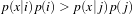 | (5.1) |
for all class j. The discriminant scores and priors are not required to be true probabilities.
This class is named the MaximumRatioDecisionRule as it can be implemented as returning the class i if
 | (5.2) |
for all class j.
We include the header files for the class as well as the header file for the std::vector class that will be the container for the discriminant scores.
The instantiation of the function is done through the usual New() method and a smart pointer.
We create the discriminant score vector and fill it with three values. We also create a vector (aPrioris) for the a priori values. The Evaluate( discriminantScores ) will return 1.
DecisionRuleType::MembershipVectorType discriminantScores;
discriminantScores.push_back( 0.1 );
discriminantScores.push_back( 0.3 );
discriminantScores.push_back( 0.6 );
DecisionRuleType::PriorProbabilityVectorType aPrioris;
aPrioris.push_back( 0.1 );
aPrioris.push_back( 0.8 );
aPrioris.push_back( 0.1 );
decisionRule->SetPriorProbabilities( aPrioris );
std::cout << "MaximumRatioDecisionRule: The index of the chosen = "
<< decisionRule->Evaluate( discriminantScores )
<< std::endl;
A random variable generation class returns a variate when the GetVariate() method is called. When we repeatedly call the method for “enough” times, the set of variates we will get follows the distribution form of the random variable generation class.
The source code for this section can be found in the file
NormalVariateGenerator.cxx.
The itk::Statistics::NormalVariateGenerator generates random variables according to the standard normal distribution (mean = 0, standard deviation = 1).
To use the class in a project, we must link the itkStatistics library to the project.
To begin the example we include the header file for the class.
The NormalVariateGenerator is a non-templated class. We simply call the New() method to create an instance. Then, we provide the seed value using the Initialize(seed value).
The source code for this section can be found in the file
ImageHistogram1.cxx.
This example shows how to compute the histogram of a scalar image. Since the statistics framework classes operate on Samples and ListOfSamples, we need to introduce a class that will make the image look like a list of samples. This class is the itk::Statistics::ImageToListSampleAdaptor. Once we have connected this adaptor to an image, we can proceed to use the itk::Statistics::SampleToHistogramFilter in order to compute the histogram of the image.
First, we need to include the headers for the itk::Statistics::ImageToListSampleAdaptor and the itk::Image classes.
Now we include the headers for the Histogram, the SampleToHistogramFilter, and the reader that we will use for reading the image from a file.
The image type must be defined using the typical pair of pixel type and dimension specification.
Using the same image type we instantiate the type of the image reader that will provide the image source for our example.
Now we introduce the central piece of this example, which is the use of the adaptor that will present the itk::Image as if it was a list of samples. We instantiate the type of the adaptor by using the actual image type. Then construct the adaptor by invoking its New() method and assigning the result to the corresponding smart pointer. Finally we connect the output of the image reader to the input of the adaptor.
You must keep in mind that adaptors are not pipeline objects. This means that they do not propagate update calls. It is therefore your responsibility to make sure that you invoke the Update() method of the reader before you attempt to use the output of the adaptor. As usual, this must be done inside a try/catch block because the read operation can potentially throw exceptions.
At this point, we are ready for instantiating the type of the histogram filter. We must first declare the type of histogram we wish to use. The adaptor type is also used as template parameter of the filter. Having instantiated this type, we proceed to create one filter by invoking its New() method.
We define now the characteristics of the Histogram that we want to compute. This typically includes the size of each one of the component, but given that in this simple example we are dealing with a scalar image, then our histogram will have a single component. For the sake of generality, however, we use the HistogramType as defined inside of the Generator type. We define also the marginal scale factor that will control the precision used when assigning values to histogram bins. Finally we invoke the Update() method in the filter.
constexpr unsigned int numberOfComponents = 1;
HistogramType::SizeType size( numberOfComponents );
size.Fill( 255 );
filter->SetInput( adaptor );
filter->SetHistogramSize( size );
filter->SetMarginalScale( 10 );
HistogramType::MeasurementVectorType min( numberOfComponents );
HistogramType::MeasurementVectorType max( numberOfComponents );
min.Fill( 0 );
max.Fill( 255 );
filter->SetHistogramBinMinimum( min );
filter->SetHistogramBinMaximum( max );
filter->Update();
Now we are ready for using the image histogram for any further processing. The histogram is obtained from the filter by invoking the GetOutput() method.
In this current example we simply print out the frequency values of all the bins in the image histogram.
The source code for this section can be found in the file
ImageHistogram2.cxx.
From the previous example you will have noticed that there is a significant number of operations to perform to compute the simple histogram of a scalar image. Given that this is a relatively common operation, it is convenient to encapsulate many of these operations in a single helper class.
The itk::Statistics::ScalarImageToHistogramGenerator is the result of such encapsulation. This example illustrates how to compute the histogram of a scalar image using this helper class.
We should first include the header of the histogram generator and the image class.
The image type must be defined using the typical pair of pixel type and dimension specification.
We use now the image type in order to instantiate the type of the corresponding histogram generator class, and invoke its New() method in order to construct one.
The image to be passed as input to the histogram generator is taken in this case from the output of an image reader.
We define also the typical parameters that specify the characteristics of the histogram to be computed.
Finally we trigger the computation of the histogram by invoking the Compute() method of the generator. Note again, that a generator is not a pipeline object and therefore it is up to you to make sure that the filters providing the input image have been updated.
The resulting histogram can be obtained from the generator by invoking its GetOutput() method. It is also convenient to get the Histogram type from the traits of the generator type itself as shown in the code below.
In this case we simply print out the frequency values of the histogram. These values can be accessed by using iterators.
The source code for this section can be found in the file
ImageHistogram3.cxx.
By now, you are probably thinking that the statistics framework in ITK is too complex for simply computing histograms from images. Here we illustrate that the benefit for this complexity is the power that these methods provide for dealing with more complex and realistic uses of image statistics than the trivial 256-bin histogram of 8-bit images that most software packages provide. One of such cases is the computation of histograms from multi-component images such as Vector images and color images.
This example shows how to compute the histogram of an RGB image by using the helper class ImageToHistogramFilter. In this first example we compute the histogram of each channel independently.
We start by including the header of the itk::Statistics::ImageToHistogramFilter, as well as the headers for the image class and the RGBPixel class.
The type of the RGB image is defined by first instantiating a RGBPixel and then using the image dimension specification.
Using the RGB image type we can instantiate the type of the corresponding histogram filter and construct one filter by invoking its New() method.
The parameters of the histogram must be defined now. Probably the most important one is the arrangement of histogram bins. This is provided to the histogram through a size array. The type of the array can be taken from the traits of the HistogramFilterType type. We create one instance of the size object and fill in its content. In this particular case, the three components of the size array will correspond to the number of bins used for each one of the RGB components in the color image. The following lines show how to define a histogram on the red component of the image while disregarding the green and blue components.
The marginal scale must be defined in the filter. This will determine the precision in the assignment of values to the histogram bins.
Finally, we must specify the upper and lower bounds for the histogram. This can either be done manually using the SetHistogramBinMinimum() and SetHistogramBinMaximum() methods or it can be done automatically by calling SetHistogramAutoMinimumMaximum( true ). Here we use the manual method.
HistogramFilterType::HistogramMeasurementVectorType lowerBound( 3 );
HistogramFilterType::HistogramMeasurementVectorType upperBound( 3 );
lowerBound[0] = 0;
lowerBound[1] = 0;
lowerBound[2] = 0;
upperBound[0] = 256;
upperBound[1] = 256;
upperBound[2] = 256;
histogramFilter->SetHistogramBinMinimum( lowerBound );
histogramFilter->SetHistogramBinMaximum( upperBound );
The input of the filter is taken from an image reader, and the computation of the histogram is triggered by invoking the Update() method of the filter.
We can now access the results of the histogram computation by declaring a pointer to histogram and getting its value from the filter using the GetOutput() method. Note that here we use a const HistogramType pointer instead of a const smart pointer because we are sure that the filter is not going to be destroyed while we access the values of the histogram. Depending on what you are doing, it may be safer to assign the histogram to a const smart pointer as shown in previous examples.
Just for the sake of exercising the experimental method [48], we verify that the resulting histogram actually have the size that we requested when we configured the filter. This can be done by invoking the Size() method of the histogram and printing out the result.
Strictly speaking, the histogram computed here is the joint histogram of the three RGB components. However, given that we set the resolution of the green and blue channels to be just one bin, the histogram is in practice representing just the red channel. In the general case, we can alway access the frequency of a particular channel in a joint histogram, thanks to the fact that the histogram class offers a GetFrequency() method that accepts a channel as argument. This is illustrated in the following lines of code.
In order to reinforce the concepts presented above, we modify now the setup of the histogram filter in order to compute the histogram of the green channel instead of the red one. This is done by simply changing the number of bins desired on each channel and invoking the computation of the filter again by calling the Update() method.
The result can be verified now by setting the desired channel to green and invoking the GetFrequency() method.
To finalize the example, we do the same computation for the case of the blue channel.
and verify the output.
The source code for this section can be found in the file
ImageHistogram4.cxx.
The statistics framework in ITK has been designed for managing multi-variate statistics in a natural way. The itk::Statistics::Histogram class reflects this concept clearly since it is a N-variable joint histogram. This nature of the Histogram class is exploited in the following example in order to build the joint histogram of a color image encoded in RGB values.
Note that the same treatment could be applied further to any vector image thanks to the generic programming approach used in the implementation of the statistical framework.
The most relevant class in this example is the itk::Statistics::ImageToHistogramFilter. This class will take care of adapting the itk::Image to a list of samples and then to a histogram filter. The user is only bound to provide the desired resolution on the histogram bins for each one of the image components.
In this example we compute the joint histogram of the three channels of an RGB image. Our output histogram will be equivalent to a 3D array of bins. This histogram could be used further for feeding a segmentation method based on statistical pattern recognition. Such method was actually used during the generation of the image in the cover of the Software Guide.
The first step is to include the header files for the histogram filter, the RGB pixel type and the Image.
We declare now the type used for the components of the RGB pixel, instantiate the type of the RGBPixel and instantiate the image type.
Using the type of the color image, and in general of any vector image, we can now instantiate the type of the histogram filter class. We then use that type for constructing an instance of the filter by invoking its New() method and assigning the result to a smart pointer.
The resolution at which the statistics of each one of the color component will be evaluated is defined by setting the number of bins along every component in the joint histogram. For this purpose we take the HistogramSizeType trait from the filter and use it to instantiate a size variable. We set in this variable the number of bins to use for each component of the color image.
Finally, we must specify the upper and lower bounds for the histogram using the SetHistogramBinMinimum() and SetHistogramBinMaximum() methods.
using HistogramMeasurementVectorType =
HistogramFilterType::HistogramMeasurementVectorType;
HistogramMeasurementVectorType binMinimum( 3 );
HistogramMeasurementVectorType binMaximum( 3 );
binMinimum[0] = -0.5;
binMinimum[1] = -0.5;
binMinimum[2] = -0.5;
binMaximum[0] = 255.5;
binMaximum[1] = 255.5;
binMaximum[2] = 255.5;
histogramFilter->SetHistogramBinMinimum( binMinimum );
histogramFilter->SetHistogramBinMaximum( binMaximum );
The input to the histogram filter is taken from the output of an image reader. Of course, the output of any filter producing an RGB image could have been used instead of a reader.
The marginal scale is defined in the histogram filter. This value will define the precision in the assignment of values to the histogram bins.
Finally, the computation of the histogram is triggered by invoking the Update() method of the filter.
At this point, we can recover the histogram by calling the GetOutput() method of the filter. The result is assigned to a variable that is instantiated using the HistogramType trait of the filter type.
We can verify that the computed histogram has the requested size by invoking its Size() method.
The values of the histogram can now be saved into a file by walking through all of the histogram bins and pushing them into a std::ofstream.
std::ofstream histogramFile;
histogramFile.open( argv[2] );
HistogramType::ConstIterator itr = histogram->Begin();
HistogramType::ConstIterator end = histogram->End();
using AbsoluteFrequencyType = HistogramType::AbsoluteFrequencyType;
while( itr != end )
{
const AbsoluteFrequencyType frequency = itr.GetFrequency();
histogramFile.write( (const char ⋆)(&frequency), sizeof(frequency) );
if (frequency != 0)
{
HistogramType::IndexType index;
index = histogram->GetIndex(itr.GetInstanceIdentifier());
std::cout << "Index = " << index << ", Frequency = " << frequency
<< std::endl;
}
++itr;
}
histogramFile.close();
Note that here the histogram is saved as a block of memory in a raw file. At this point you can use visualization software in order to explore the histogram in a display that would be equivalent to a scatter plot of the RGB components of the input color image.
Many concepts from Information Theory have been used successfully in the domain of image processing. This section introduces some of such concepts and illustrates how the statistical framework in ITK can be used for computing measures that have some relevance in terms of Information Theory [57, 58, 32].
The concept of Entropy has been introduced into image processing as a crude mapping from its application in Communications. The notions of Information Theory can be deceiving and misleading when applied to images because their language from Communication Theory does not necessarily map to what people in the Imaging Community use.
For example, it is commonly said that
“The Entropy of an image is a measure of the amount of information contained in an image”.
This statement is fundamentally incorrect.
The way the notion of Entropy is commonly measured in images is by first assuming that the spatial location of a pixel in an image is irrelevant! That is, we simply take the statistical distribution of the pixel values as it can be evaluated in a histogram and from that histogram we estimate the frequency of the value associated to each bin. In other words, we simply assume that the image is a set of pixels that are passing through a channel, just as things are commonly considered for communication purposes.
Once the frequency of every pixel value has been estimated, Information Theory defines that the amount of uncertainty that an observer will lose by taking one pixel and finding its real value to be the one associated with the i-th bin of the histogram, is given by -log2(pi), where pi is the frequency in that histogram bin. Since a reduction in uncertainty is equivalent to an increase in the amount of information in the observer, we conclude that measuring one pixel and finding its level to be in the i-th bin results in an acquisition of -log2(pi) bits of information1 .
Since we could have picked any pixel at random, our chances of picking the ones that are associated to the i-th histogram bin are given by pi. Therefore, the expected reduction in uncertainty that we can get from measuring the value of one pixel is given by
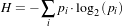 | (5.3) |
This quantity H is what is usually defined as the Entropy of the Image. It would be more accurate to call it the Entropy of the random variable associated to the intensity value of one pixel. The fact that H is unrelated to the spatial arrangement of the pixels in an image shows how little of the real Image Information H actually represents. The Entropy of an image, as measured above, is only a crude indication of how the intensity values are spread in the dynamic range of intensities. For example, an image with maximum entropy will be the one that has a large dynamic range and every value in that range is equally probable.
The common convention of H as a representation of image information has terribly undermined the enormous potential on the application of Information Theory to image processing and analysis.
The real concepts of Information Theory would require that we define the amount of information in an image based on our expectations and prior knowledge from that image. In particular, the Amount of Information provided by an image should measure the number of features that we are not able to predict based on our prior knowledge about that image. For example, if we know that we are going to analyze a CT scan of the abdomen of an adult human male in the age range of 40 to 45, there is already a good deal that we could predict about the content of that image. The real amount of information in the image is the representation of the features in the image that we could not predict from knowing that it is a CT scan from a human adult male.
The application of Information Theory to image analysis is still in its early infancy and it is an exciting and promising field to be explored further. All that being said, let’s now look closer at how the concept of Entropy (which is not the amount of information in an image) can be measured with the ITK statistics framework.
The source code for this section can be found in the file
ImageEntropy1.cxx.
This example shows how to compute the entropy of an image. More formally this should be said : The reduction in uncertainty gained when we measure the intensity of one randomly selected pixel in this image, given that we already know the statistical distribution of the image intensity values.
In practice it is almost never possible to know the real statistical distribution of intensities and we are forced to estimate it from the evaluation of the histogram from one or several images of similar nature. We can use the counts in histogram bins in order to compute frequencies and then consider those frequencies to be estimations of the probablility of a new value to belong to the intensity range of that bin.
Since the first stage in estimating the entropy of an image is to compute its histogram, we must start by including the headers of the classes that will perform such a computation. In this case, we are going to use a scalar image as input, therefore we need the itk::Statistics::ScalarImageToHistogramGenerator class, as well as the image class.
The pixel type and dimension of the image are explicitly declared and then used for instantiating the image type.
The image type is used as template parameter for instantiating the histogram generator.
The parameters of the desired histogram are defined, including the number of bins and the marginal scale. For convenience in this example, we read the number of bins from the command line arguments. In this way we can easily experiment with different values for the number of bins and see how that choice affects the computation of the entropy.
We can then connect as input the output image from a reader and trigger the histogram computation by invoking the Compute() method in the generator.
The resulting histogram can be recovered from the generator by using the GetOutput() method. A histogram class can be declared using the HistogramType trait from the generator.
We proceed now to compute the estimation of entropy given the histogram. The first conceptual jump to be done here is to assume that the histogram, which is the simple count of frequency of occurrence for the gray scale values of the image pixels, can be normalized in order to estimate the probability density function PDF of the actual statistical distribution of pixel values.
First we declare an iterator that will visit all the bins in the histogram. Then we obtain the total number of counts using the GetTotalFrequency() method, and we initialize the entropy variable to zero.
We start now visiting every bin and estimating the probability of a pixel to have a value in the range of that bin. The base 2 logarithm of that probability is computed, and then weighted by the probability in order to compute the expected amount of information for any given pixel. Note that a minimum value is imposed for the probability in order to avoid computing logarithms of zeros.
Note that the log(2) factor is used to convert the natural logarithm in to a logarithm of base 2, and makes it possible to report the entropy in its natural unit: the bit.
The result of this sum is considered to be our estimation of the image entropy. Note that the Entropy value will change depending on the number of histogram bins that we use for computing the histogram. This is particularly important when dealing with images whose pixel values have dynamic ranges so large that our number of bins will always underestimate the variability of the data.
As an illustration, the application of this program to the image
results in the following values of entropy for different values of number of histogram bins.
| Number of Histogram Bins | 16 | 32 | 64 | 128 | 255 |
| Estimated Entropy (bits) | 3.02 | 3.98 | 4.92 | 5.89 | 6.88 |
This table highlights the importance of carefully considering the characteristics of the histograms used for estimating Information Theory measures such as the entropy.
The source code for this section can be found in the file
ImageMutualInformation1.cxx.
This example illustrates how to compute the Mutual Information between two images using classes from the Statistics framework. Note that you could also use for this purpose the ImageMetrics designed for the image registration framework.
For example, you could use:
Mutual Information as computed in this example, and as commonly used in the context of image registration provides a measure of how much uncertainty on the value of a pixel in one image is reduced by measuring the homologous pixel in the other image. Note that Mutual Information as used here does not measure the amount of information that one image provides on the other image; this would require us to take into account the spatial structures in the images as well as the semantics of the image context in terms of an observer.
This implies that there is still an enormous unexploited potential on the use of the Mutual Information concept in the domain of medical images, among the most interesting of which is the semantic description of image in terms of anatomical structures.
In this particular example we make use of classes from the Statistics framework in order to compute the measure of Mutual Information between two images. We assume that both images have the same number of pixels along every dimension and that they have the same origin and spacing. Therefore the pixels from one image are perfectly aligned with those of the other image.
We must start by including the header files of the image, histogram filter, reader and Join image filter. We will read both images and use the Join image filter in order to compose an image of two components using the information of each one of the input images in one component. This is the natural way of using the Statistics framework in ITK given that the fundamental statistical classes are expecting to receive multi-valued measures.
We define the pixel type and dimension of the images to be read.
Using the image type we proceed to instantiate the readers for both input images. Then, we take their filenames from the command line arguments.
Using the itk::JoinImageFilter we use the two input images and put them together in an image of two components.
At this point we trigger the execution of the pipeline by invoking the Update() method on the Join filter. We must put the call inside a try/catch block because the Update() call may potentially result in exceptions being thrown.
We now prepare the types to be used for the computation of the joint histogram. For this purpose, we take the type of the image resulting from the JoinImageFilter and use it as template argument of the itk::ImageToHistogramFilter. We then construct one by invoking the New() method.
We pass the multiple-component image as input to the histogram filter, and setup the marginal scale value that will define the precision to be used for classifying values into the histogram bins.
We must now define the number of bins to use for each one of the components in the joint image. For this purpose we take the HistogramSizeType from the traits of the histogram filter type.
Finally, we must specify the upper and lower bounds for the histogram using the SetHistogramBinMinimum() and SetHistogramBinMaximum() methods. The Update() method is then called in order to trigger the computation of the histogram.
using HistogramMeasurementVectorType =
HistogramFilterType::HistogramMeasurementVectorType;
HistogramMeasurementVectorType binMinimum( 3 );
HistogramMeasurementVectorType binMaximum( 3 );
binMinimum[0] = -0.5;
binMinimum[1] = -0.5;
binMinimum[2] = -0.5;
binMaximum[0] = 255.5;
binMaximum[1] = 255.5;
binMaximum[2] = 255.5;
histogramFilter->SetHistogramBinMinimum( binMinimum );
histogramFilter->SetHistogramBinMaximum( binMaximum );
histogramFilter->Update();
The histogram can be recovered from the filter by creating a variable with the histogram type taken from the filter traits.
We now walk over all the bins of the joint histogram and compute their contribution to the value of the joint entropy. For this purpose we use histogram iterators, and the Begin() and End() methods. Since the values returned from the histogram are measuring frequency we must convert them to an estimation of probability by dividing them over the total sum of frequencies returned by the GetTotalFrequency() method.
We initialize to zero the variable to use for accumulating the value of the joint entropy, and then use the iterator for visiting all the bins of the joint histogram. For every bin we compute their contribution to the reduction of uncertainty. Note that in order to avoid logarithmic operations on zero values, we skip over those bins that have less than one count. The entropy contribution must be computed using logarithms in base two in order to express entropy in bits.
Now that we have the value of the joint entropy we can proceed to estimate the values of the entropies for each image independently. This can be done by simply changing the number of bins and then recomputing the histogram.
We initialize to zero another variable in order to start accumulating the entropy contributions from every bin.
The same process is used for computing the entropy of the other component, simply by swapping the number of bins in the histogram.
The entropy is computed in a similar manner, just by visiting all the bins on the histogram and accumulating their entropy contributions.
At this point we can compute any of the popular measures of Mutual Information. For example
or Normalized Mutual Information, where the value of Mutual Information is divided by the mean entropy of the input images.
A second form of Normalized Mutual Information has been defined as the mean entropy of the two images divided by their joint entropy.
You probably will find very interesting how the value of Mutual Information is strongly dependent on the number of bins over which the histogram is defined.
In statistical classification, each object is represented by d features (a measurement vector), and the goal of classification becomes finding compact and disjoint regions (decision regions[18]) for classes in a d-dimensional feature space. Such decision regions are defined by decision rules that are known or can be trained. The simplest configuration of a classification consists of a decision rule and multiple membership functions; each membership function represents a class. Figure 5.3 illustrates this general framework.
This framework closely follows that of Duda and Hart[18]. The classification process can be described as follows:
This simple configuration can be used to formulated various classification tasks by using different membership functions and incorporating task specific requirements and prior knowledge into the decision rule. For example, instead of using probability density functions as membership functions, through distance functions and a minimum value decision rule (which assigns a class from the distance function that returns the smallest value) users can achieve a least squared error classifier. As another example, users can add a rejection scheme to the decision rule so that even in a situation where the membership scores suggest a “winner”, a measurement vector can be flagged as ill-defined. Such a rejection scheme can avoid risks of assigning a class label without a proper win margin.
The source code for this section can be found in the file
KdTreeBasedKMeansClustering.cxx.
K-means clustering is a popular clustering algorithm because it is simple and usually converges to a reasonable solution. The k-means algorithm works as follows:
The most common termination criterion is that if there is no measurement vector that changes its cluster membership from the previous iteration, then the algorithm stops.
The itk::Statistics::KdTreeBasedKmeansEstimator is a variation of this logic. The k-means clustering algorithm is computationally very expensive because it has to recalculate the mean at each iteration. To update the mean values, we have to calculate the distance between k means and each and every measurement vector. To reduce the computational burden, the KdTreeBasedKmeansEstimator uses a special data structure: the k-d tree ( itk::Statistics::KdTree) with additional information. The additional information includes the number and the vector sum of measurement vectors under each node under the tree architecture.
With such additional information and the k-d tree data structure, we can reduce the computational cost of the distance calculation and means. Instead of calculating each measurement vector and k means, we can simply compare each node of the k-d tree and the k means. This idea of utilizing a k-d tree can be found in multiple articles [2] [44] [28]. Our implementation of this scheme follows the article by the Kanungo et al [28].
We use the itk::Statistics::ListSample as the input sample, the itk::Vector as the measurement vector. The following code snippet includes their header files.
Since our k-means algorithm requires a itk::Statistics::KdTree object as an input, we include the KdTree class header file. As mentioned above, we need a k-d tree with the vector sum and the number of measurement vectors. Therefore we use the itk::Statistics::WeightedCentroidKdTreeGenerator instead of the itk::Statistics::KdTreeGenerator that generate a k-d tree without such additional information.
The KdTreeBasedKmeansEstimator class is the implementation of the k-means algorithm. It does not create k clusters. Instead, it returns the mean estimates for the k clusters.
To generate the clusters, we must create k instances of
itk::Statistics::DistanceToCentroidMembershipFunction function as the membership functions
for each cluster and plug that—along with a sample—into an itk::Statistics::SampleClassifierFilter
object to get a itk::Statistics::MembershipSample that stores pairs of measurement vectors and their
associated class labels (k labels).
We will fill the sample with random variables from two normal distribution using the itk::Statistics::NormalVariateGenerator.
Since the NormalVariateGenerator class only supports 1-D, we define our measurement vector type as one component vector. We then, create a ListSample object for data inputs. Each measurement vector is of length 1. We set this using the SetMeasurementVectorSize() method.
The following code snippet creates a NormalVariateGenerator object. Since the random variable generator returns values according to the standard normal distribution (The mean is zero, and the standard deviation is one), before pushing random values into the sample, we change the mean and standard deviation. We want two normal (Gaussian) distribution data. We have two for loops. Each for loop uses different mean and standard deviation. Before we fill the sample with the second distribution data, we call Initialize(random seed) method, to recreate the pool of random variables in the normalGenerator.
To see the probability density plots from the two distribution, refer to the Figure 5.5.
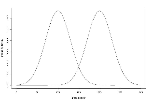
using NormalGeneratorType = itk::Statistics::NormalVariateGenerator;
NormalGeneratorType::Pointer normalGenerator = NormalGeneratorType::New();
normalGenerator->Initialize( 101 );
MeasurementVectorType mv;
double mean = 100;
double standardDeviation = 30;
for (unsigned int i = 0; i < 100; ++i)
{
mv[0] = ( normalGenerator->GetVariate() ⋆ standardDeviation ) + mean;
sample->PushBack( mv );
}
normalGenerator->Initialize( 3024 );
mean = 200;
standardDeviation = 30;
for (unsigned int i = 0; i < 100; ++i)
{
mv[0] = ( normalGenerator->GetVariate() ⋆ standardDeviation ) + mean;
sample->PushBack( mv );
}
We create a k-d tree. To see the details on the k-d tree generation, see the Section 5.1.7.
Once we have the k-d tree, it is a simple procedure to produce k mean estimates.
We create the KdTreeBasedKmeansEstimator. Then, we provide the initial mean values using the SetParameters(). Since we are dealing with two normal distribution in a 1-D space, the size of the mean value array is two. The first element is the first mean value, and the second is the second mean value. If we used two normal distributions in a 2-D space, the size of array would be four, and the first two elements would be the two components of the first normal distribution’s mean vector. We plug-in the k-d tree using the SetKdTree().
The remaining two methods specify the termination condition. The estimation process stops when the number of iterations reaches the maximum iteration value set by the SetMaximumIteration(), or the distances between the newly calculated mean (centroid) values and previous ones are within the threshold set by the SetCentroidPositionChangesThreshold(). The final step is to call the StartOptimization() method.
The for loop will print out the mean estimates from the estimation process.
using TreeType = TreeGeneratorType::KdTreeType;
using EstimatorType = itk::Statistics::KdTreeBasedKmeansEstimator<TreeType>;
EstimatorType::Pointer estimator = EstimatorType::New();
EstimatorType::ParametersType initialMeans(2);
initialMeans[0] = 0.0;
initialMeans[1] = 0.0;
estimator->SetParameters( initialMeans );
estimator->SetKdTree( treeGenerator->GetOutput() );
estimator->SetMaximumIteration( 200 );
estimator->SetCentroidPositionChangesThreshold(0.0);
estimator->StartOptimization();
EstimatorType::ParametersType estimatedMeans = estimator->GetParameters();
for (unsigned int i = 0; i < 2; ++i)
{
std::cout << "cluster[" << i << "] " << std::endl;
std::cout << " estimated mean : " << estimatedMeans[i] << std::endl;
}
If we are only interested in finding the mean estimates, we might stop. However, to illustrate how a classifier can be formed using the statistical classification framework. We go a little bit further in this example.
Since the k-means algorithm is an minimum distance classifier using the estimated k means and the measurement vectors. We use the DistanceToCentroidMembershipFunction class as membership functions. Our choice for the decision rule is the itk::Statistics::MinimumDecisionRule that returns the index of the membership functions that have the smallest value for a measurement vector.
After creating a SampleClassifier filter object and a MinimumDecisionRule object, we plug-in the decisionRule and the sample to the classifier filter. Then, we must specify the number of classes that will be considered using the SetNumberOfClasses() method.
The remainder of the following code snippet shows how to use user-specified class labels. The classification result will be stored in a MembershipSample object, and for each measurement vector, its class label will be one of the two class labels, 100 and 200 (unsigned int).
using MembershipFunctionType =
itk::Statistics::DistanceToCentroidMembershipFunction
<MeasurementVectorType>;
using DecisionRuleType = itk::Statistics::MinimumDecisionRule;
DecisionRuleType::Pointer decisionRule = DecisionRuleType::New();
using ClassifierType = itk::Statistics::SampleClassifierFilter< SampleType >;
ClassifierType::Pointer classifier = ClassifierType::New();
classifier->SetDecisionRule( decisionRule );
classifier->SetInput( sample );
classifier->SetNumberOfClasses( 2 );
using ClassLabelVectorObjectType =
ClassifierType::ClassLabelVectorObjectType;
using ClassLabelVectorType =
ClassifierType::ClassLabelVectorType;
using ClassLabelType =
ClassifierType::ClassLabelType;
ClassLabelVectorObjectType::Pointer classLabelsObject =
ClassLabelVectorObjectType::New();
ClassLabelVectorType& classLabelsVector = classLabelsObject->Get();
ClassLabelType class1 = 200;
classLabelsVector.push_back( class1 );
ClassLabelType class2 = 100;
classLabelsVector.push_back( class2 );
classifier->SetClassLabels( classLabelsObject );
The classifier is almost ready to do the classification process except that it needs two membership functions that represents two clusters respectively.
In this example, the two clusters are modeled by two Euclidean distance functions. The distance function (model) has only one parameter, its mean (centroid) set by the SetCentroid() method. To plug-in two distance functions, we create a MembershipFunctionVectorObject that contains a MembershipFunctionVector with two components and add it using the SetMembershipFunctions method. Then invocation of the Update() method will perform the classification.
using MembershipFunctionVectorObjectType =
ClassifierType::MembershipFunctionVectorObjectType;
using MembershipFunctionVectorType =
ClassifierType::MembershipFunctionVectorType;
MembershipFunctionVectorObjectType::Pointer membershipFunctionVectorObject =
MembershipFunctionVectorObjectType::New();
MembershipFunctionVectorType& membershipFunctionVector =
membershipFunctionVectorObject->Get();
int index = 0;
for (unsigned int i = 0; i < 2; i++)
{
MembershipFunctionType::Pointer membershipFunction
= MembershipFunctionType::New();
MembershipFunctionType::CentroidType centroid(
sample->GetMeasurementVectorSize() );
for ( unsigned int j = 0; j < sample->GetMeasurementVectorSize(); j++ )
{
centroid[j] = estimatedMeans[index++];
}
membershipFunction->SetCentroid( centroid );
membershipFunctionVector.push_back( membershipFunction );
}
classifier->SetMembershipFunctions( membershipFunctionVectorObject );
classifier->Update();
The following code snippet prints out the measurement vectors and their class labels in the sample.
const ClassifierType::MembershipSampleType⋆ membershipSample =
classifier->GetOutput();
ClassifierType::MembershipSampleType::ConstIterator iter
= membershipSample->Begin();
while ( iter != membershipSample->End() )
{
std::cout << "measurement vector = " << iter.GetMeasurementVector()
<< " class label = " << iter.GetClassLabel()
<< std::endl;
++iter;
}
The source code for this section can be found in the file
ScalarImageKmeansClassifier.cxx.
This example shows how to use the KMeans model for classifying the pixel of a scalar image.
The itk::Statistics::ScalarImageKmeansImageFilter is used for taking a scalar image and applying the K-Means algorithm in order to define classes that represents statistical distributions of intensity values in the pixels. The classes are then used in this filter for generating a labeled image where every pixel is assigned to one of the classes.
First we define the pixel type and dimension of the image that we intend to classify. With this image type we can also declare the itk::ImageFileReader needed for reading the input image, create one and set its input filename.
With the ImageType we instantiate the type of the itk::ScalarImageKmeansImageFilter that will compute the K-Means model and then classify the image pixels.
In general the classification will produce as output an image whose pixel values are integers associated to the labels of the classes. Since typically these integers will be generated in order (0,1,2,...N), the output image will tend to look very dark when displayed with naive viewers. It is therefore convenient to have the option of spreading the label values over the dynamic range of the output image pixel type. When this is done, the dynamic range of the pixels is divided by the number of classes in order to define the increment between labels. For example, an output image of 8 bits will have a dynamic range of [0:256], and when it is used for holding four classes, the non-contiguous labels will be (0,64,128,192). The selection of the mode to use is done with the method SetUseNonContiguousLabels().
For each one of the classes we must provide a tentative initial value for the mean of the class. Given that this is a scalar image, each one of the means is simply a scalar value. Note however that in a general case of K-Means, the input image would be a vector image and therefore the means will be vectors of the same dimension as the image pixels.
The itk::ScalarImageKmeansImageFilter is predefined for producing an 8 bits scalar image as output. This output image contains labels associated to each one of the classes in the K-Means algorithm. In the following lines we use the OutputImageType in order to instantiate the type of a itk::ImageFileWriter. Then create one, and connect it to the output of the classification filter.
We are now ready for triggering the execution of the pipeline. This is done by simply invoking the Update() method in the writer. This call will propagate the update request to the reader and then to the classifier.
At this point the classification is done, the labeled image is saved in a file, and we can take a look at the means that were found as a result of the model estimation performed inside the classifier filter.
KMeansFilterType::ParametersType estimatedMeans =
kmeansFilter->GetFinalMeans();
const unsigned int numberOfClasses = estimatedMeans.Size();
for ( unsigned int i = 0; i < numberOfClasses; ++i )
{
std::cout << "cluster[" << i << "] ";
std::cout << " estimated mean : " << estimatedMeans[i] << std::endl;
}
Figure 5.6 illustrates the effect of this filter with three classes. The means were estimated by ScalarImageKmeansModelEstimator.cxx.
The source code for this section can be found in the file
BayesianPluginClassifier.cxx.
In this example, we present a system that places measurement vectors into two Gaussian classes. The Figure 5.7 shows all the components of the classifier system and the data flow. This system differs with the previous k-means clustering algorithms in several ways. The biggest difference is that this classifier uses the itk::Statistics::GaussianDensityFunctions as membership functions instead of the itk::Statistics::DistanceToCentroidMembershipFunction. Since the membership function is different, the membership function requires a different set of parameters, mean vectors and covariance matrices. We choose the itk::Statistics::CovarianceSampleFilter (sample covariance) for the estimation algorithms of the two parameters. If we want a more robust estimation algorithm, we can replace this estimation algorithm with more alternatives without changing other components in the classifier system.
It is a bad idea to use the same sample for test and training (parameter estimation) of the parameters. However, for simplicity, in this example, we use a sample for test and training.
We use the itk::Statistics::ListSample as the sample (test and training). The itk::Vector is our measurement vector class. To store measurement vectors into two separate sample containers, we use the itk::Statistics::Subsample objects.
The following file provides us the parameter estimation algorithm.
The following files define the components required by ITK statistical classification framework: the decision rule, the membership function, and the classifier.
We will fill the sample with random variables from two normal distribution using the itk::Statistics::NormalVariateGenerator.
Since the NormalVariateGenerator class only supports 1-D, we define our measurement vector type as a one component vector. We then, create a ListSample object for data inputs.
We also create two Subsample objects that will store the measurement vectors in sample into two separate sample containers. Each Subsample object stores only the measurement vectors belonging to a single class. This class sample will be used by the parameter estimation algorithms.
constexpr unsigned int measurementVectorLength = 1;
using MeasurementVectorType = itk::Vector< double, measurementVectorLength >;
using SampleType = itk::Statistics::ListSample< MeasurementVectorType >;
SampleType::Pointer sample = SampleType::New();
// length of measurement vectors in the sample.
sample->SetMeasurementVectorSize( measurementVectorLength );
using ClassSampleType = itk::Statistics::Subsample< SampleType >;
std::vector< ClassSampleType::Pointer > classSamples;
for ( unsigned int i = 0; i < 2; ++i )
{
classSamples.push_back( ClassSampleType::New() );
classSamples[i]->SetSample( sample );
}
The following code snippet creates a NormalVariateGenerator object. Since the random variable generator returns values according to the standard normal distribution (the mean is zero, and the standard deviation is one) before pushing random values into the sample, we change the mean and standard deviation. We want two normal (Gaussian) distribution data. We have two for loops. Each for loop uses different mean and standard deviation. Before we fill the sample with the second distribution data, we call Initialize(random seed) method, to recreate the pool of random variables in the normalGenerator. In the second for loop, we fill the two class samples with measurement vectors using the AddInstance() method.
To see the probability density plots from the two distributions, refer to Figure 5.5.
using NormalGeneratorType = itk::Statistics::NormalVariateGenerator;
NormalGeneratorType::Pointer normalGenerator = NormalGeneratorType::New();
normalGenerator->Initialize( 101 );
MeasurementVectorType mv;
double mean = 100;
double standardDeviation = 30;
SampleType::InstanceIdentifier id = 0UL;
for ( unsigned int i = 0; i < 100; ++i )
{
mv.Fill( (normalGenerator->GetVariate() ⋆ standardDeviation ) + mean);
sample->PushBack( mv );
classSamples[0]->AddInstance( id );
++id;
}
normalGenerator->Initialize( 3024 );
mean = 200;
standardDeviation = 30;
for ( unsigned int i = 0; i < 100; ++i )
{
mv.Fill( (normalGenerator->GetVariate() ⋆ standardDeviation ) + mean);
sample->PushBack( mv );
classSamples[1]->AddInstance( id );
++id;
}
In the following code snippet, notice that the template argument for the CovarianceCalculator is ClassSampleType (i.e., type of Subsample) instead of SampleType (i.e., type of ListSample). This is because the parameter estimation algorithms are applied to the class sample.
using CovarianceEstimatorType =
itk::Statistics::CovarianceSampleFilter<ClassSampleType>;
std::vector< CovarianceEstimatorType::Pointer > covarianceEstimators;
for ( unsigned int i = 0; i < 2; ++i )
{
covarianceEstimators.push_back( CovarianceEstimatorType::New() );
covarianceEstimators[i]->SetInput( classSamples[i] );
covarianceEstimators[i]->Update();
}
We print out the estimated parameters.
After creating a SampleClassifier object and a MaximumRatioDecisionRule object, we plug in the decisionRule and the sample to the classifier. Then, we specify the number of classes that will be considered using the SetNumberOfClasses() method.
The MaximumRatioDecisionRule requires a vector of a priori probability values. Such a priori probability will be the P(ωi) of the following variation of the Bayes decision rule:
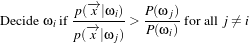 | (5.4) |
The remainder of the code snippet shows how to use user-specified class labels. The classification result will be stored in a MembershipSample object, and for each measurement vector, its class label will be one of the two class labels, 100 and 200 (unsigned int).
using MembershipFunctionType =
itk::Statistics::GaussianMembershipFunction<MeasurementVectorType>;
using DecisionRuleType = itk::Statistics::MaximumRatioDecisionRule;
DecisionRuleType::Pointer decisionRule = DecisionRuleType::New();
DecisionRuleType::PriorProbabilityVectorType aPrioris;
aPrioris.push_back( (double)classSamples[0]->GetTotalFrequency()
/ (double)sample->GetTotalFrequency() );
aPrioris.push_back( (double)classSamples[1]->GetTotalFrequency()
/ (double)sample->GetTotalFrequency() );
decisionRule->SetPriorProbabilities( aPrioris );
using ClassifierType = itk::Statistics::SampleClassifierFilter< SampleType >;
ClassifierType::Pointer classifier = ClassifierType::New();
classifier->SetDecisionRule( decisionRule);
classifier->SetInput( sample );
classifier->SetNumberOfClasses( 2 );
using ClassLabelVectorObjectType =
ClassifierType::ClassLabelVectorObjectType;
using ClassLabelVectorType = ClassifierType::ClassLabelVectorType;
ClassLabelVectorObjectType::Pointer classLabelVectorObject =
ClassLabelVectorObjectType::New();
ClassLabelVectorType classLabelVector = classLabelVectorObject->Get();
ClassifierType::ClassLabelType class1 = 100;
classLabelVector.push_back( class1 );
ClassifierType::ClassLabelType class2 = 200;
classLabelVector.push_back( class2 );
classLabelVectorObject->Set( classLabelVector );
classifier->SetClassLabels( classLabelVectorObject );
The classifier is almost ready to perform the classification except that it needs two membership functions that represent the two clusters.
In this example, we can imagine that the two clusters are modeled by two Gaussian distribution functions. The distribution functions have two parameters, the mean, set by the SetMean() method, and the covariance, set by the SetCovariance() method. To plug-in two distribution functions, we create a new instance of MembershipFunctionVectorObjectType and populate its internal vector with new instances of MembershipFunction (i.e. GaussianMembershipFunction). This is done by calling the Get() method of membershipFunctionVectorObject to get the internal vector, populating this vector with two new membership functions and then calling membershipFunctionVectorObject->Set( membershipFunctionVector ). Finally, the invocation of the Update() method will perform the classification.
using MembershipFunctionVectorObjectType =
ClassifierType::MembershipFunctionVectorObjectType;
using MembershipFunctionVectorType =
ClassifierType::MembershipFunctionVectorType;
MembershipFunctionVectorObjectType::Pointer membershipFunctionVectorObject =
MembershipFunctionVectorObjectType::New();
MembershipFunctionVectorType membershipFunctionVector =
membershipFunctionVectorObject->Get();
for (unsigned int i = 0; i < 2; ++i)
{
MembershipFunctionType::Pointer membershipFunction =
MembershipFunctionType::New();
membershipFunction->SetMean( covarianceEstimators[i]->GetMean() );
membershipFunction->SetCovariance(
covarianceEstimators[i]->GetCovarianceMatrix() );
membershipFunctionVector.push_back( membershipFunction );
}
membershipFunctionVectorObject->Set( membershipFunctionVector );
classifier->SetMembershipFunctions( membershipFunctionVectorObject );
classifier->Update();
The following code snippet prints out pairs of a measurement vector and its class label in the sample.
const ClassifierType::MembershipSampleType⋆ membershipSample
= classifier->GetOutput();
ClassifierType::MembershipSampleType::ConstIterator iter
= membershipSample->Begin();
while ( iter != membershipSample->End() )
{
std::cout << "measurement vector = " << iter.GetMeasurementVector()
<< " class label = " << iter.GetClassLabel() << std::endl;
++iter;
}
The source code for this section can be found in the file
ExpectationMaximizationMixtureModelEstimator.cxx.
In this example, we present an implementation of the expectation maximization (EM) process to generates parameter estimates for a two Gaussian component mixture model.
The Bayesian plug-in classifier example (see Section 5.4.3) used two Gaussian probability density functions (PDF) to model two Gaussian distribution classes (two models for two class). However, in some cases, we want to model a distribution as a mixture of several different distributions. Therefore, the probability density function (p(x)) of a mixture model can be stated as follows :
 | (5.5) |
where i is the index of the component, c is the number of components, αi is the proportion of the component, and fi is the probability density function of the component.
Now the task is to find the parameters(the component PDF’s parameters and the proportion values) to maximize the likelihood of the parameters. If we know which component a measurement vector belongs to, the solutions to this problem is easy to solve. However, we don’t know the membership of each measurement vector. Therefore, we use the expectation of membership instead of the exact membership. The EM process splits into two steps:
The E step is basically a step that calculates the a posteriori probability for each measurement vector.
The M step is dependent on the type of each PDF. Most of distributions belonging to exponential family such as Poisson, Binomial, Exponential, and Normal distributions have analytical solutions for updating the parameter set. The itk::Statistics::ExpectationMaximizationMixtureModelEstimator class assumes that such type of components.
In the following example we use the itk::Statistics::ListSample as the sample (test and training). The itk::Vector::is our measurement vector class. To store measurement vectors into two separate sample container, we use the itk::Statistics::Subsample objects.
The following two files provides us the parameter estimation algorithms.
We will fill the sample with random variables from two normal distribution using the itk::Statistics::NormalVariateGenerator.
Since the NormalVariateGenerator class only supports 1-D, we define our measurement vector type as a one component vector. We then, create a ListSample object for data inputs.
We also create two Subsample objects that will store the measurement vectors in the sample into two separate sample containers. Each Subsample object stores only the measurement vectors belonging to a single class. This class sample will be used by the parameter estimation algorithms.
unsigned int numberOfClasses = 2;
using MeasurementVectorType = itk::Vector< double, 1 >;
using SampleType = itk::Statistics::ListSample< MeasurementVectorType >;
SampleType::Pointer sample = SampleType::New();
sample->SetMeasurementVectorSize( 1 ); // length of measurement vectors
// in the sample.
The following code snippet creates a NormalVariateGenerator object. Since the random variable generator returns values according to the standard normal distribution (the mean is zero, and the standard deviation is one) before pushing random values into the sample, we change the mean and standard deviation. We want two normal (Gaussian) distribution data. We have two for loops. Each for loop uses different mean and standard deviation. Before we fill the sample with the second distribution data, we call Initialize() method to recreate the pool of random variables in the normalGenerator. In the second for loop, we fill the two class samples with measurement vectors using the AddInstance() method.
To see the probability density plots from the two distribution, refer to Figure 5.5.
using NormalGeneratorType = itk::Statistics::NormalVariateGenerator;
NormalGeneratorType::Pointer normalGenerator = NormalGeneratorType::New();
normalGenerator->Initialize( 101 );
MeasurementVectorType mv;
double mean = 100;
double standardDeviation = 30;
for ( unsigned int i = 0; i < 100; ++i )
{
mv[0] = ( normalGenerator->GetVariate() ⋆ standardDeviation ) + mean;
sample->PushBack( mv );
}
normalGenerator->Initialize( 3024 );
mean = 200;
standardDeviation = 30;
for ( unsigned int i = 0; i < 100; ++i )
{
mv[0] = ( normalGenerator->GetVariate() ⋆ standardDeviation ) + mean;
sample->PushBack( mv );
}
In the following code snippet notice that the template argument for the MeanCalculator and CovarianceCalculator is ClassSampleType (i.e., type of Subsample) instead of SampleType (i.e., type of ListSample). This is because the parameter estimation algorithms are applied to the class sample.
using ParametersType = itk::Array< double >;
ParametersType params( 2 );
std::vector< ParametersType > initialParameters( numberOfClasses );
params[0] = 110.0;
params[1] = 800.0;
initialParameters[0] = params;
params[0] = 210.0;
params[1] = 850.0;
initialParameters[1] = params;
using ComponentType =
itk::Statistics::GaussianMixtureModelComponent<SampleType>;
std::vector< ComponentType::Pointer > components;
for ( unsigned int i = 0; i < numberOfClasses; i++ )
{
components.push_back( ComponentType::New() );
(components[i])->SetSample( sample );
(components[i])->SetParameters( initialParameters[i] );
}
We run the estimator.
using EstimatorType =
itk::Statistics::ExpectationMaximizationMixtureModelEstimator<SampleType>;
EstimatorType::Pointer estimator = EstimatorType::New();
estimator->SetSample( sample );
estimator->SetMaximumIteration( 200 );
itk::Array< double > initialProportions(numberOfClasses);
initialProportions[0] = 0.5;
initialProportions[1] = 0.5;
estimator->SetInitialProportions( initialProportions );
for (unsigned int i = 0; i < numberOfClasses; ++i)
{
estimator->AddComponent( (ComponentType::Superclass⋆)
(components[i]).GetPointer() );
}
estimator->Update();
We then print out the estimated parameters.
for (unsigned int i = 0; i < numberOfClasses; ++i)
{
std::cout << "Cluster[" << i << "]" << std::endl;
std::cout << " Parameters:" << std::endl;
std::cout << " " << (components[i])->GetFullParameters()
<< std::endl;
std::cout << " Proportion: ";
std::cout << " " << estimator->GetProportions()[i] << std::endl;
}
Markov Random Fields are probabilistic models that use the correlation between pixels in a neighborhood to decide the object region. The itk::Statistics::MRFImageFilter uses the maximum a posteriori (MAP) estimates for modeling the MRF. The object traverses the data set and uses the model generated by the Mahalanobis distance classifier to gets the the distance between each pixel in the data set to a set of known classes, updates the distances by evaluating the influence of its neighboring pixels (based on a MRF model) and finally, classifies each pixel to the class which has the minimum distance to that pixel (taking the neighborhood influence under consideration). The energy function minimization is done using the iterated conditional modes (ICM) algorithm [6].
The source code for this section can be found in the file
ScalarImageMarkovRandomField1.cxx.
This example shows how to use the Markov Random Field approach for classifying the pixel of a scalar image.
The itk::Statistics::MRFImageFilter is used for refining an initial classification by introducing the spatial coherence of the labels. The user should provide two images as input. The first image is the one to be classified while the second image is an image of labels representing an initial classification.
The following headers are related to reading input images, writing the output image, and making the necessary conversions between scalar and vector images.
The following headers are related to the statistical classification classes.
First we define the pixel type and dimension of the image that we intend to classify. With this image type we can also declare the itk::ImageFileReader needed for reading the input image, create one and set its input filename. In this particular case we choose to use signed short as pixel type, which is typical for MicroMRI and CT data sets.
As a second step we define the pixel type and dimension of the image of labels that provides the initial classification of the pixels from the first image. This initial labeled image can be the output of a K-Means method like the one illustrated in section 5.4.2.
Since the Markov Random Field algorithm is defined in general for images whose pixels have multiple components, that is, images of vector type, we must adapt our scalar image in order to satisfy the interface expected by the MRFImageFilter. We do this by using the itk::ComposeImageFilter. With this filter we will present our scalar image as a vector image whose vector pixels contain a single component.
using ArrayPixelType = itk::FixedArray<LabelPixelType,1>;
using ArrayImageType = itk::Image< ArrayPixelType, Dimension >;
using ScalarToArrayFilterType = itk::ComposeImageFilter<
ImageType, ArrayImageType >;
ScalarToArrayFilterType::Pointer
scalarToArrayFilter = ScalarToArrayFilterType::New();
scalarToArrayFilter->SetInput( reader->GetOutput() );
With the input image type ImageType and labeled image type LabelImageType we instantiate the type of the itk::MRFImageFilter that will apply the Markov Random Field algorithm in order to refine the pixel classification.
We set now some of the parameters for the MRF filter. In particular, the number of classes to be used during the classification, the maximum number of iterations to be run in this filter and the error tolerance that will be used as a criterion for convergence.
The smoothing factor represents the tradeoff between fidelity to the observed image and the smoothness of the segmented image. Typical smoothing factors have values between 1 5. This factor will multiply the weights that define the influence of neighbors on the classification of a given pixel. The higher the value, the more uniform will be the regions resulting from the classification refinement.
Given that the MRF filter need to continually relabel the pixels, it needs access to a set of membership functions that will measure to what degree every pixel belongs to a particular class. The classification is performed by the itk::ImageClassifierBase class, that is instantiated using the type of the input vector image and the type of the labeled image.
The classifier need a decision rule to be set by the user. Note that we must use GetPointer() in the call of the SetDecisionRule() method because we are passing a SmartPointer, and smart pointer cannot perform polymorphism, we must then extract the raw pointer that is associated to the smart pointer. This extraction is done with the GetPointer() method.
We now instantiate the membership functions. In this case we use the itk::Statistics::DistanceToCentroidMembershipFunction class templated over the pixel type of the vector image, that in our example happens to be a vector of dimension 1.
using MembershipFunctionType =
itk::Statistics::DistanceToCentroidMembershipFunction<ArrayPixelType>;
using MembershipFunctionPointer = MembershipFunctionType::Pointer;
double meanDistance = 0;
MembershipFunctionType::CentroidType centroid(1);
for( unsigned int i=0; i < numberOfClasses; i++ )
{
MembershipFunctionPointer membershipFunction =
MembershipFunctionType::New();
centroid[0] = std::stod( argv[i+numberOfArgumentsBeforeMeans] );
membershipFunction->SetCentroid( centroid );
classifier->AddMembershipFunction( membershipFunction );
meanDistance += static_cast< double > (centroid[0]);
}
if (numberOfClasses > 0)
{
meanDistance /= numberOfClasses;
}
else
{
std::cerr << "ERROR: numberOfClasses is 0" << std::endl;
return EXIT_FAILURE;
}
We set the Smoothing factor. This factor will multiply the weights that define the influence of neighbors on the classification of a given pixel. The higher the value, the more uniform will be the regions resulting from the classification refinement.
and we set the neighborhood radius that will define the size of the clique to be used in the computation of the neighbors’ influence in the classification of any given pixel. Note that despite the fact that we call this a radius, it is actually the half size of an hypercube. That is, the actual region of influence will not be circular but rather an N-Dimensional box. For example, a neighborhood radius of 2 in a 3D image will result in a clique of size 5x5x5 pixels, and a radius of 1 will result in a clique of size 3x3x3 pixels.
We should now set the weights used for the neighbors. This is done by passing an array of values that contains the linear sequence of weights for the neighbors. For example, in a neighborhood of size 3x3x3, we should provide a linear array of 9 weight values. The values are packaged in a std::vector and are supposed to be double. The following lines illustrate a typical set of values for a 3x3x3 neighborhood. The array is arranged and then passed to the filter by using the method SetMRFNeighborhoodWeight().
We now scale weights so that the smoothing function and the image fidelity functions have comparable value. This is necessary since the label image and the input image can have different dynamic ranges. The fidelity function is usually computed using a distance function, such as the itk::DistanceToCentroidMembershipFunction or one of the other membership functions. They tend to have values in the order of the means specified.
double totalWeight = 0;
for(std::vector< double >::const_iterator wcIt = weights.begin();
wcIt != weights.end(); ++wcIt )
{
totalWeight += ⋆wcIt;
}
for(double & weight : weights)
{
weight =
static_cast< double > ( weight ⋆ meanDistance / (2 ⋆ totalWeight));
}
mrfFilter->SetMRFNeighborhoodWeight( weights );
Finally, the classifier class is connected to the Markof Random Fields filter.
The output image produced by the itk::MRFImageFilter has the same pixel type as the labeled input image. In the following lines we use the OutputImageType in order to instantiate the type of a itk::ImageFileWriter. Then create one, and connect it to the output of the classification filter after passing it through an intensity rescaler to rescale it to an 8 bit dynamic range
We are now ready for triggering the execution of the pipeline. This is done by simply invoking the Update() method in the writer. This call will propagate the update request to the reader and then to the MRF filter.
Figure 5.8 illustrates the effect of this filter with three classes. In this example the filter was run with a smoothing factor of 3. The labeled image was produced by ScalarImageKmeansClassifier.cxx and the means were estimated by ScalarImageKmeansModelEstimator.cxx.