![I(X) ∈[low er,upper]](ITKSoftwareGuide-Book2309x.png)
Segmentation of medical images is a challenging task. A myriad of different methods have been proposed and implemented in recent years. In spite of the huge effort invested in this problem, there is no single approach that can generally solve the problem of segmentation for the large variety of image modalities existing today.
The most effective segmentation algorithms are obtained by carefully customizing combinations of components. The parameters of these components are tuned for the characteristics of the image modality used as input and the features of the anatomical structure to be segmented.
The Insight Toolkit provides a basic set of algorithms that can be used to develop and customize a full segmentation application. Some of the most commonly used segmentation components are described in the following sections.
Region growing algorithms have proven to be an effective approach for image segmentation. The basic approach of a region growing algorithm is to start from a seed region (typically one or more pixels) that are considered to be inside the object to be segmented. The pixels neighboring this region are evaluated to determine if they should also be considered part of the object. If so, they are added to the region and the process continues as long as new pixels are added to the region. Region growing algorithms vary depending on the criteria used to decide whether a pixel should be included in the region or not, the type connectivity used to determine neighbors, and the strategy used to visit neighboring pixels.
Several implementations of region growing are available in ITK. This section describes some of the most commonly used.
A simple criterion for including pixels in a growing region is to evaluate intensity value inside a specific interval.
The source code for this section can be found in the file
ConnectedThresholdImageFilter.cxx.
The following example illustrates the use of the itk::ConnectedThresholdImageFilter. This filter uses the flood fill iterator. Most of the algorithmic complexity of a region growing method comes from visiting neighboring pixels. The flood fill iterator assumes this responsibility and greatly simplifies the implementation of the region growing algorithm. Thus the algorithm is left to establish a criterion to decide whether a particular pixel should be included in the current region or not.
The criterion used by the ConnectedThresholdImageFilter is based on an interval of intensity values provided by the user. Lower and upper threshold values should be provided. The region-growing algorithm includes those pixels whose intensities are inside the interval.
|
| (4.1) |
Let’s look at the minimal code required to use this algorithm. First, the following header defining the ConnectedThresholdImageFilter class must be included.
Noise present in the image can reduce the capacity of this filter to grow large regions. When faced with noisy images, it is usually convenient to pre-process the image by using an edge-preserving smoothing filter. Any of the filters discussed in Section 2.7.3 could be used to this end. In this particular example we use the itk::CurvatureFlowImageFilter, so we need to include its header file.
We declare the image type based on a particular pixel type and dimension. In this case the float type is used for the pixels due to the requirements of the smoothing filter.
The smoothing filter is instantiated using the image type as a template parameter.
Then the filter is created by invoking the New() method and assigning the result to a itk::SmartPointer.
We now declare the type of the region growing filter. In this case it is the ConnectedThresholdImageFilter.
Then we construct one filter of this class using the New() method.
Now it is time to connect a simple, linear pipeline. A file reader is added at the beginning of the pipeline and a cast filter and writer are added at the end. The cast filter is required to convert float pixel types to integer types since only a few image file formats support float types.
CurvatureFlowImageFilter requires a couple of parameters. The following are typical values for 2D images. However, these values may have to be adjusted depending on the amount of noise present in the input image.
We now set the lower and upper threshold values. Any pixel whose value is between lowerThreshold and upperThreshold will be included in the region, and any pixel whose value is outside will be excluded. Setting these values too close together will be too restrictive for the region to grow; setting them too far apart will cause the region to engulf the image.
The output of this filter is a binary image with zero-value pixels everywhere except on the extracted region. The intensity value set inside the region is selected with the method SetReplaceValue().
The algorithm must be initialized by setting a seed point (i.e., the itk::Index of the pixel from which the region will grow) using the SetSeed() method. It is convenient to initialize with a point in a typical region of the anatomical structure to be segmented.
Invocation of the Update() method on the writer triggers execution of the pipeline. It is usually wise to put update calls in a try/catch block in case errors occur and exceptions are thrown.
Let’s run this example using as input the image BrainProtonDensitySlice.png provided in the directory Examples/Data. We can easily segment the major anatomical structures by providing seeds in the appropriate locations and defining values for the lower and upper thresholds. Figure 4.1 illustrates several examples of segmentation. The parameters used are presented in Table 4.1.
Notice that the gray matter is not being completely segmented. This illustrates the vulnerability of the region-growing methods when the anatomical structures to be segmented do not have a homogeneous statistical distribution over the image space. You may want to experiment with different values of the lower and upper thresholds to verify how the accepted region will extend.
Another option for segmenting regions is to take advantage of the functionality provided by the ConnectedThresholdImageFilter for managing multiple seeds. The seeds can be passed one-by-one to the filter using the AddSeed() method. You could imagine a user interface in which an operator clicks on multiple points of the object to be segmented and each selected point is passed as a seed to this filter.
Another criterion for classifying pixels is to minimize the error of misclassification. The goal is to find a threshold that classifies the image into two clusters such that we minimize the area under the histogram for one cluster that lies on the other cluster’s side of the threshold. This is equivalent to minimizing the within class variance or equivalently maximizing the between class variance.
The source code for this section can be found in the file
OtsuThresholdImageFilter.cxx.
This example illustrates how to use the itk::OtsuThresholdImageFilter.
The next step is to decide which pixel types to use for the input and output images, and to define the image dimension.
The input and output image types are now defined using their respective pixel types and dimensions.
The filter type can be instantiated using the input and output image types defined above.
An itk::ImageFileReader class is also instantiated in order to read image data from a file. (See Section 1 on page 3 for more information about reading and writing data.)
An itk::ImageFileWriter is instantiated in order to write the output image to a file.
Both the filter and the reader are created by invoking their New() methods and assigning the result to itk::SmartPointers.
The image obtained with the reader is passed as input to the OtsuThresholdImageFilter.
The method SetOutsideValue() defines the intensity value to be assigned to those pixels whose intensities are outside the range defined by the lower and upper thresholds. The method SetInsideValue() defines the intensity value to be assigned to pixels with intensities falling inside the threshold range.
Execution of the filter is triggered by invoking the Update() method, which we wrap in a try/catch block. If the filter’s output has been passed as input to subsequent filters, the Update() call on any downstream filters in the pipeline will indirectly trigger the update of this filter.
We can now retrieve the internally-computed threshold value with the GetThreshold() method and print it to the console.

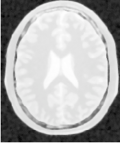
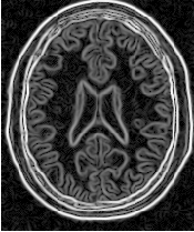
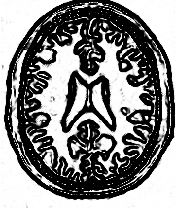
Figure 4.2 illustrates the effect of this filter on a MRI proton density image of the brain. This figure shows the limitations of this filter for performing segmentation by itself. These limitations are particularly noticeable in noisy images and in images lacking spatial uniformity as is the case with MRI due to field bias.
The following classes provide similar functionality:
The source code for this section can be found in the file
OtsuMultipleThresholdImageFilter.cxx.
This example illustrates how to use the itk::OtsuMultipleThresholdsCalculator.
OtsuMultipleThresholdsCalculator calculates thresholds for a given histogram so as to maximize the between-class variance. We use ScalarImageToHistogramGenerator to generate histograms. The histogram type defined by the generator is then used to instantiate the type of the Otsu threshold calculator.
Once thresholds are computed we will use BinaryThresholdImageFilter to segment the input image.
Create a histogram generator and calculator using the standard New() method.
Set the following properties for the histogram generator and the calculators, in this case grabbing the number of thresholds from the command line.
The pipeline will look as follows:
Here we obtain a const reference to the thresholds by calling the GetOutput() method.
We now iterate through thresholdVector, printing each value to the console and writing an image thresholded with adjacent values from the container. (In the edge cases, the minimum and maximum values of the InternalPixelType are used).
Also write out the image thresholded between the upper threshold and the max intensity.
The source code for this section can be found in the file
NeighborhoodConnectedImageFilter.cxx.
The following example illustrates the use of the itk::NeighborhoodConnectedImageFilter. This filter is a close variant of the itk::ConnectedThresholdImageFilter. On one hand, the ConnectedThresholdImageFilter considers only the value of the pixel itself when determining whether it belongs to the region: if its value is within the interval [lowerThreshold,upperThreshold] it is included, otherwise it is excluded. NeighborhoodConnectedImageFilter, on the other hand, considers a user-defined neighborhood surrounding the pixel, requiring that the intensity of each neighbor be within the interval for it to be included.
The reason for considering the neighborhood intensities instead of only the current pixel intensity is that small structures are less likely to be accepted in the region. The operation of this filter is equivalent to applying ConnectedThresholdImageFilter followed by mathematical morphology erosion using a structuring element of the same shape as the neighborhood provided to the NeighborhoodConnectedImageFilter.
The itk::CurvatureFlowImageFilter is used here to smooth the image while preserving edges.
We now define the image type using a particular pixel type and image dimension. In this case the float type is used for the pixels due to the requirements of the smoothing filter.
The smoothing filter type is instantiated using the image type as a template parameter.
Then, the filter is created by invoking the New() method and assigning the result to a itk::SmartPointer.
We now declare the type of the region growing filter. In this case it is the NeighborhoodConnectedImageFilter.
One filter of this class is constructed using the New() method.
Now it is time to create a simple, linear data processing pipeline. A file reader is added at the beginning of the pipeline and a cast filter and writer are added at the end. The cast filter is required to convert float pixel types to integer types since only a few image file formats support float types.
CurvatureFlowImageFilter requires a couple of parameters. The following are typical values for 2D images. However, they may have to be adjusted depending on the amount of noise present in the input image.
NeighborhoodConnectedImageFilter requires that two main parameters are specified. They are the lower and upper thresholds of the interval in which intensity values must fall to be included in the region. Setting these two values too close will not allow enough flexibility for the region to grow. Setting them too far apart will result in a region that engulfs the image.
Here, we add the crucial parameter that defines the neighborhood size used to determine whether a pixel lies in the region. The larger the neighborhood, the more stable this filter will be against noise in the input image, but also the longer the computing time will be. Here we select a filter of radius 2 along each dimension. This results in a neighborhood of 5×5 pixels.
As in the ConnectedThresholdImageFilter example, we must provide the intensity value to be used for the output pixels accepted in the region and at least one seed point to define the starting point.
Invocation of the Update() method on the writer triggers the execution of the pipeline. It is usually wise to put update calls in a try/catch block in case errors occur and exceptions are thrown.
Now we’ll run this example using the image BrainProtonDensitySlice.png as input available from the directory Examples/Data. We can easily segment the major anatomical structures by providing seeds in the appropriate locations and defining values for the lower and upper thresholds. For example
As with the ConnectedThresholdImageFilter example, several seeds could be provided to the filter by repetedly calling the AddSeed() method with different indices. Compare Figures 4.3 and 4.1, demonstrating the outputs of NeighborhoodConnectedThresholdImageFilter and ConnectedThresholdImageFilter, respectively. It is instructive to adjust the neighborhood radii and observe its effect on the smoothness of segmented object borders, size of the segmented region, and computing time.
The source code for this section can be found in the file
ConfidenceConnected.cxx.
The following example illustrates the use of the itk::ConfidenceConnectedImageFilter. The criterion used by the ConfidenceConnectedImageFilter is based on simple statistics of the current region. First, the algorithm computes the mean and standard deviation of intensity values for all the pixels currently included in the region. A user-provided factor is used to multiply the standard deviation and define a range around the mean. Neighbor pixels whose intensity values fall inside the range are accepted and included in the region. When no more neighbor pixels are found that satisfy the criterion, the algorithm is considered to have finished its first iteration. At that point, the mean and standard deviation of the intensity levels are recomputed using all the pixels currently included in the region. This mean and standard deviation defines a new intensity range that is used to visit current region neighbors and evaluate whether their intensity falls inside the range. This iterative process is repeated until no more pixels are added or the maximum number of iterations is reached. The following equation illustrates the inclusion criterion used by this filter,
![I(X)∈ [m - fσ,m+ fσ]](ITKSoftwareGuide-Book2320x.png) | (4.2) |
where m and σ are the mean and standard deviation of the region intensities, f is a factor defined by the user, I() is the image and X is the position of the particular neighbor pixel being considered for inclusion in the region.
Let’s look at the minimal code required to use this algorithm. First, the following header defining the itk::ConfidenceConnectedImageFilter class must be included.
Noise present in the image can reduce the capacity of this filter to grow large regions. When faced with noisy images, it is usually convenient to pre-process the image by using an edge-preserving smoothing filter. Any of the filters discussed in Section 2.7.3 can be used to this end. In this particular example we use the itk::CurvatureFlowImageFilter, hence we need to include its header file.
We now define the image type using a pixel type and a particular dimension. In this case the float type is used for the pixels due to the requirements of the smoothing filter.
The smoothing filter type is instantiated using the image type as a template parameter.
Next the filter is created by invoking the New() method and assigning the result to a itk::SmartPointer.
We now declare the type of the region growing filter. In this case it is the ConfidenceConnectedImageFilter.
Then, we construct one filter of this class using the New() method.
Now it is time to create a simple, linear pipeline. A file reader is added at the beginning of the pipeline and a cast filter and writer are added at the end. The cast filter is required here to convert float pixel types to integer types since only a few image file formats support float types.
CurvatureFlowImageFilter requires two parameters. The following are typical values for 2D images. However they may have to be adjusted depending on the amount of noise present in the input image.
ConfidenceConnectedImageFilter also requires two parameters. First, the factor f defines how large the range of intensities will be. Small values of the multiplier will restrict the inclusion of pixels to those having very similar intensities to those in the current region. Larger values of the multiplier will relax the accepting condition and will result in more generous growth of the region. Values that are too large will cause the region to grow into neighboring regions which may belong to separate anatomical structures. This is not desirable behavior.
The number of iterations is specified based on the homogeneity of the intensities of the anatomical structure to be segmented. Highly homogeneous regions may only require a couple of iterations. Regions with ramp effects, like MRI images with inhomogeneous fields, may require more iterations. In practice, it seems to be more important to carefully select the multiplier factor than the number of iterations. However, keep in mind that there is no guarantee that this algorithm will converge on a stable region. It is possible that by letting the algorithm run for more iterations the region will end up engulfing the entire image.
The output of this filter is a binary image with zero-value pixels everywhere except on the extracted region. The intensity value to be set inside the region is selected with the method SetReplaceValue().
The initialization of the algorithm requires the user to provide a seed point. It is convenient to select this point to be placed in a typical region of the anatomical structure to be segmented. A small neighborhood around the seed point will be used to compute the initial mean and standard deviation for the inclusion criterion. The seed is passed in the form of an itk::Index to the SetSeed() method.
The size of the initial neighborhood around the seed is defined with the method SetInitialNeighborhoodRadius(). The neighborhood will be defined as an N-dimensional rectangular region with 2r+1 pixels on the side, where r is the value passed as initial neighborhood radius.
The invocation of the Update() method on the writer triggers the execution of the pipeline. It is recommended to place update calls in a try/catch block in case errors occur and exceptions are thrown.
Let’s now run this example using as input the image BrainProtonDensitySlice.png provided in the directory Examples/Data. We can easily segment the major anatomical structures by providing seeds in the appropriate locations. For example
Note that the gray matter is not being completely segmented. This illustrates the vulnerability of the region growing methods when the anatomical structures to be segmented do not have a homogeneous statistical distribution over the image space. You may want to experiment with different numbers of iterations to verify how the accepted region will extend.
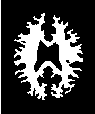
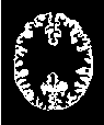
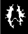
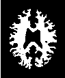
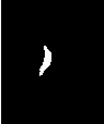
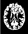
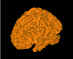
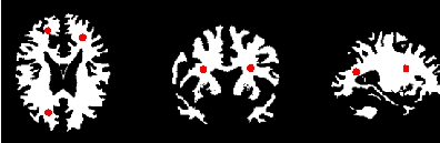
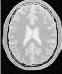
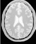
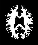
This section shows some results obtained by applying the Confidence Connected filter on the BrainWeb database. The filter was applied on a 181 × 217 × 181 crosssection of the brainweb165a10f17 dataset. The data is a MR T1 acquisition, with an intensity non-uniformity of 20% and a slice thickness 1mm. The dataset may be obtained from http://www.bic.mni.mcgill.ca/brainweb/ or https://data.kitware.com/#folder/5882712d8d777f4f3f3072df
The previous code was used in this example replacing the image dimension by 3. Gradient Anistropic diffusion was applied to smooth the image. The filter used 2 iterations, a time step of 0.05 and a conductance value of 3. The smoothed volume was then segmented using the Confidence Connected approach. Five seed points were used at coordinate locations (118,85,92), (63,87,94), (63,157,90), (111,188,90), (111,50,88). The ConfidenceConnnected filter used the parameters, a neighborhood radius of 2, 5 iterations and an f of 2.5 (the same as in the previous example). The results were then rendered using VolView.
Figure 4.5 shows the rendered volume. Figure 4.6 shows an axial, saggital and a coronal slice of the volume.
The source code for this section can be found in the file
IsolatedConnectedImageFilter.cxx.
The following example illustrates the use of the itk::IsolatedConnectedImageFilter. This filter is a close variant of the itk::ConnectedThresholdImageFilter. In this filter two seeds and a lower threshold are provided by the user. The filter will grow a region connected to the first seed and not connected to the second one. In order to do this, the filter finds an intensity value that could be used as upper threshold for the first seed. A binary search is used to find the value that separates both seeds.
This example closely follows the previous ones. Only the relevant pieces of code are highlighted here.
The header of the IsolatedConnectedImageFilter is included below.
We define the image type using a pixel type and a particular dimension.
The IsolatedConnectedImageFilter is instantiated in the lines below.
One filter of this class is constructed using the New() method.
Now it is time to connect the pipeline.
The IsolatedConnectedImageFilter expects the user to specify a threshold and two seeds. In this example, we take all of them from the command line arguments.
As in the itk::ConnectedThresholdImageFilter we must now specify the intensity value to be set on the output pixels and at least one seed point to define the initial region.
The invocation of the Update() method on the writer triggers the execution of the pipeline.
The intensity value allowing us to separate both regions can be recovered with the method GetIsolatedValue().
Let’s now run this example using the image BrainProtonDensitySlice.png provided in the directory Examples/Data. We can easily segment the major anatomical structures by providing seed pairs in the appropriate locations and defining values for the lower threshold. It is important to keep in mind in this and the previous examples that the segmentation is being performed using the smoothed version of the image. The selection of threshold values should therefore be performed in the smoothed image since the distribution of intensities could be quite different from that of the input image. As a reminder of this fact, Figure 4.7 presents, from left to right, the input image and the result of smoothing with the itk::CurvatureFlowImageFilter followed by segmentation results.
This filter is intended to be used in cases where adjacent anatomical structures are difficult to separate. Selecting one seed in one structure and the other seed in the adjacent structure creates the appropriate setup for computing the threshold that will separate both structures. Table 4.2 presents the parameters used to obtain the images shown in Figure 4.7.
| Adjacent Structures | Seed1 | Seed2 | Lower | Isolated value found |
| Gray matter vs White matter | (61,140) | (63,43) | 150 | 183.31 |
The source code for this section can be found in the file
VectorConfidenceConnected.cxx.
This example illustrates the use of the confidence connected concept applied to images with vector pixel types. The confidence connected algorithm is implemented for vector images in the class itk::VectorConfidenceConnected. The basic difference between the scalar and vector version is that the vector version uses the covariance matrix instead of a variance, and a vector mean instead of a scalar mean. The membership of a vector pixel value to the region is measured using the Mahalanobis distance as implemented in the class itk::Statistics::MahalanobisDistanceThresholdImageFunction.
We now define the image type using a particular pixel type and dimension. In this case the float type is used for the pixels due to the requirements of the smoothing filter.
We now declare the type of the region-growing filter. In this case it is the itk::VectorConfidenceConnectedImageFilter.
Then, we construct one filter of this class using the New() method.
Next we create a simple, linear data processing pipeline.
VectorConfidenceConnectedImageFilter requires two parameters. First, the multiplier factor f defines how large the range of intensities will be. Small values of the multiplier will restrict the inclusion of pixels to those having similar intensities to those already in the current region. Larger values of the multiplier relax the accepting condition and result in more generous growth of the region. Values that are too large will cause the region to grow into neighboring regions which may actually belong to separate anatomical structures.
The number of iterations is typically determined based on the homogeneity of the image intensity representing the anatomical structure to be segmented. Highly homogeneous regions may only require a couple of iterations. Regions with ramp effects, like MRI images with inhomogeneous fields, may require more iterations. In practice, it seems to be more relevant to carefully select the multiplier factor than the number of iterations. However, keep in mind that there is no reason to assume that this algorithm should converge to a stable region. It is possible that by letting the algorithm run for more iterations the region will end up engulfing the entire image.
The output of this filter is a binary image with zero-value pixels everywhere except on the extracted region. The intensity value to be put inside the region is selected with the method SetReplaceValue().
The initialization of the algorithm requires the user to provide a seed point. This point should be placed in a typical region of the anatomical structure to be segmented. A small neighborhood around the seed point will be used to compute the initial mean and standard deviation for the inclusion criterion. The seed is passed in the form of an itk::Index to the SetSeed() method.
The size of the initial neighborhood around the seed is defined with the method SetInitialNeighborhoodRadius(). The neighborhood will be defined as an N-Dimensional rectangular region with 2r+1 pixels on the side, where r is the value passed as initial neighborhood radius.
The invocation of the Update() method on the writer triggers the execution of the pipeline. It is usually wise to put update calls in a try/catch block in case errors occur and exceptions are thrown.
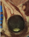
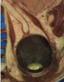
Now let’s run this example using as input the image VisibleWomanEyeSlice.png provided in the directory Examples/Data. We can easily segment the major anatomical structures by providing seeds in the appropriate locations. For example,
The coloration of muscular tissue makes it easy to distinguish them from the surrounding anatomical structures. The optic vitrea on the other hand has a coloration that is not very homogeneous inside the eyeball and does not facilitate a full segmentation based only on color.
The values of the final mean vector and covariance matrix used for the last iteration can be queried using the methods GetMean() and GetCovariance().
using MeanVectorType = ConnectedFilterType::MeanVectorType;
using CovarianceMatrixType = ConnectedFilterType::CovarianceMatrixType;
const MeanVectorType & mean = confidenceConnected->GetMean();
const CovarianceMatrixType & covariance
= confidenceConnected->GetCovariance();
std::cout << "Mean vector = " << mean << std::endl;
std::cout << "Covariance matrix = " << covariance << std::endl;
Watershed segmentation classifies pixels into regions using gradient descent on image features and analysis of weak points along region boundaries. Imagine water raining onto a landscape topology and flowing with gravity to collect in low basins. The size of those basins will grow with increasing amounts of precipitation until they spill into one another, causing small basins to merge together into larger basins. Regions (catchment basins) are formed by using local geometric structure to associate points in the image domain with local extrema in some feature measurement such as curvature or gradient magnitude. This technique is less sensitive to user-defined thresholds than classic region-growing methods, and may be better suited for fusing different types of features from different data sets. The watersheds technique is also more flexible in that it does not produce a single image segmentation, but rather a hierarchy of segmentations from which a single region or set of regions can be extracted a-priori, using a threshold, or interactively, with the help of a graphical user interface [73, 74].
The strategy of watershed segmentation is to treat an image f as a height function, i.e., the surface formed
by graphing f as a function of its independent parameters,  ∈ U. The image f is often not the original input
data, but is derived from that data through some filtering, graded (or fuzzy) feature extraction, or fusion of
feature maps from different sources. The assumption is that higher values of f (or -f) indicate the presence
of boundaries in the original data. Watersheds may therefore be considered as a final or intermediate step in
a hybrid segmentation method, where the initial segmentation is the generation of the edge feature
map.
∈ U. The image f is often not the original input
data, but is derived from that data through some filtering, graded (or fuzzy) feature extraction, or fusion of
feature maps from different sources. The assumption is that higher values of f (or -f) indicate the presence
of boundaries in the original data. Watersheds may therefore be considered as a final or intermediate step in
a hybrid segmentation method, where the initial segmentation is the generation of the edge feature
map.
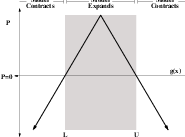
Gradient descent associates regions with local minima of f (clearly interior points) using the watersheds of the graph of f, as in Figure 4.9.
That is, a segment consists of all points in U whose paths of steepest descent on the graph of f terminate at the same minimum in f. Thus, there are as many segments in an image as there are minima in f. The segment boundaries are “ridges” [29, 30, 19] in the graph of f. In the 1D case (U ⊂ℜ), the watershed boundaries are the local maxima of f, and the results of the watershed segmentation is trivial. For higher-dimensional image domains, the watershed boundaries are not simply local phenomena; they depend on the shape of the entire watershed.
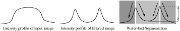
The drawback of watershed segmentation is that it produces a region for each local minimum—in practice too many regions—and an over segmentation results. To alleviate this, we can establish a minimum watershed depth. The watershed depth is the difference in height between the watershed minimum and the lowest boundary point. In other words, it is the maximum depth of water a region could hold without flowing into any of its neighbors. Thus, a watershed segmentation algorithm can sequentially combine watersheds whose depths fall below the minimum until all of the watersheds are of sufficient depth. This depth measurement can be combined with other saliency measurements, such as size. The result is a segmentation containing regions whose boundaries and size are significant. Because the merging process is sequential, it produces a hierarchy of regions, as shown in Figure 4.10.
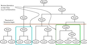
Previous work has shown the benefit of a user-assisted approach that provides a graphical interface to this hierarchy, so that a technician can quickly move from the small regions that lie within an area of interest to the union of regions that correspond to the anatomical structure [74].
There are two different algorithms commonly used to implement watersheds: top-down and bottom-up. The top-down, gradient descent strategy was chosen for ITK because we want to consider the output of multi-scale differential operators, and the f in question will therefore have floating point values. The bottom-up strategy starts with seeds at the local minima in the image and grows regions outward and upward at discrete intensity levels (equivalent to a sequence of morphological operations and sometimes called morphological watersheds [55].) This limits the accuracy by enforcing a set of discrete gray levels on the image.
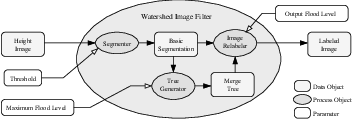
Figure 4.11 shows how the ITK image-to-image watersheds filter is constructed. The filter is actually a collection of smaller filters that modularize the several steps of the algorithm in a mini-pipeline. The segmenter object creates the initial segmentation via steepest descent from each pixel to local minima. Shallow background regions are removed (flattened) before segmentation using a simple minimum value threshold (this helps to minimize oversegmentation of the image). The initial segmentation is passed to a second sub-filter that generates a hierarchy of basins to a user-specified maximum watershed depth. The relabeler object at the end of the mini-pipeline uses the hierarchy and the initial segmentation to produce an output image at any scale below the user-specified maximum. Data objects are cached in the mini-pipeline so that changing watershed depths only requires a (fast) relabeling of the basic segmentation. The three parameters that control the filter are shown in Figure 4.11 connected to their relevant processing stages.
The source code for this section can be found in the file
WatershedSegmentation1.cxx.
The following example illustrates how to preprocess and segment images using the itk::WatershedImageFilter. Note that the care with which the data are preprocessed will greatly affect the quality of your result. Typically, the best results are obtained by preprocessing the original image with an edge-preserving diffusion filter, such as one of the anisotropic diffusion filters, or the bilateral image filter. As noted in Section 4.2.1, the height function used as input should be created such that higher positive values correspond to object boundaries. A suitable height function for many applications can be generated as the gradient magnitude of the image to be segmented.
The itk::VectorGradientMagnitudeAnisotropicDiffusionImageFilter class is used to smooth the image and the itk::VectorGradientMagnitudeImageFilter is used to generate the height function. We begin by including all preprocessing filter header files and the header file for the WatershedImageFilter. We use the vector versions of these filters because the input dataset is a color image.
We now declare the image and pixel types to use for instantiation of the filters. All of these filters expect real-valued pixel types in order to work properly. The preprocessing stages are applied directly to the vector-valued data and the segmentation uses floating point scalar data. Images are converted from RGB pixel type to numerical vector type using itk::CastImageFilter.
using RGBPixelType = itk::RGBPixel< unsigned char >;
using RGBImageType = itk::Image< RGBPixelType, 2 >;
using VectorPixelType = itk::Vector< float, 3 >;
using VectorImageType = itk::Image< VectorPixelType, 2 >;
using LabeledImageType = itk::Image< itk::IdentifierType, 2 >;
using ScalarImageType = itk::Image< float, 2 >;
The various image processing filters are declared using the types created above and eventually used in the pipeline.
using FileReaderType = itk::ImageFileReader< RGBImageType >;
using CastFilterType = itk::CastImageFilter< RGBImageType, VectorImageType >;
using DiffusionFilterType =
itk::VectorGradientAnisotropicDiffusionImageFilter<
VectorImageType, VectorImageType >;
using GradientMagnitudeFilterType =
itk::VectorGradientMagnitudeImageFilter<VectorImageType>;
using WatershedFilterType = itk::WatershedImageFilter<ScalarImageType>;
Next we instantiate the filters and set their parameters. The first step in the image processing pipeline is diffusion of the color input image using an anisotropic diffusion filter. For this class of filters, the CFL condition requires that the time step be no more than 0.25 for two-dimensional images, and no more than 0.125 for three-dimensional images. The number of iterations and the conductance term will be taken from the command line. See Section 2.7.3 for more information on the ITK anisotropic diffusion filters.
The ITK gradient magnitude filter for vector-valued images can optionally take several parameters. Here we allow only enabling or disabling of principal component analysis.
Finally we set up the watershed filter. There are two parameters. Level controls watershed depth, and Threshold controls the lower thresholding of the input. Both parameters are set as a percentage (0.0 - 1.0) of the maximum depth in the input image.
The output of WatershedImageFilter is an image of unsigned long integer labels, where a label denotes membership of a pixel in a particular segmented region. This format is not practical for visualization, so for the purposes of this example, we will convert it to RGB pixels. RGB images have the advantage that they can be saved as a simple png file and viewed using any standard image viewer software. The itk::Functor::ScalarToRGBPixelFunctor class is a special function object designed to hash a scalar value into an itk::RGBPixel. Plugging this functor into the itk::UnaryFunctorImageFilter creates an image filter which converts scalar images to RGB images.
The filters are connected into a single pipeline, with readers and writers at each end.

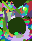
Tuning the filter parameters for any particular application is a process of trial and error. The threshold parameter can be used to great effect in controlling oversegmentation of the image. Raising the threshold will generally reduce computation time and produce output with fewer and larger regions. The trick in tuning parameters is to consider the scale level of the objects that you are trying to segment in the image. The best time/quality trade-off will be achieved when the image is smoothed and thresholded to eliminate features just below the desired scale.
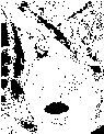
Figure 4.12 shows output from the example code. The input image is taken from the Visible Human female data around the right eye. The images on the right are colorized watershed segmentations with parameters set to capture objects such as the optic nerve and lateral rectus muscles, which can be seen just above and to the left and right of the eyeball. Note that a critical difference between the two segmentations is the mode of the gradient magnitude calculation.
A note on the computational complexity of the watershed algorithm is warranted. Most of the complexity of the ITK implementation lies in generating the hierarchy. Processing times for this stage are non-linear with respect to the number of catchment basins in the initial segmentation. This means that the amount of information contained in an image is more significant than the number of pixels in the image. A very large, but very flat input take less time to segment than a very small, but very detailed input.
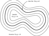
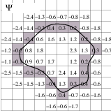
Figure 4.13: Concept of zero set in a level set.
The paradigm of the level set is that it is a numerical method for tracking the evolution of contours and surfaces. Instead of manipulating the contour directly, the contour is embedded as the zero level set of a higher dimensional function called the level-set function, ψ(X,t). The level-set function is then evolved under the control of a differential equation. At any time, the evolving contour can be obtained by extracting the zero level-set Γ(X,t) = {ψ(X,t) = 0} from the output. The main advantages of using level sets is that arbitrarily complex shapes can be modeled and topological changes such as merging and splitting are handled implicitly.
Level sets can be used for image segmentation by using image-based features such as mean intensity, gradient and edges in the governing differential equation. In a typical approach, a contour is initialized by a user and is then evolved until it fits the form of an anatomical structure in the image. Many different implementations and variants of this basic concept have been published in the literature. An overview of the field has been made by Sethian [56].
The following sections introduce practical examples of some of the level set segmentation methods available in ITK. The remainder of this section describes features common to all of these filters except the itk::FastMarchingImageFilter, which is derived from a different code framework. Understanding these features will aid in using the filters more effectively.
Each filter makes use of a generic level-set equation to compute the update to the solution ψ of the partial differential equation.
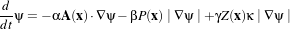 | (4.3) |
where A is an advection term, P is a propagation (expansion) term, and Z is a spatial modifier term for the mean curvature κ. The scalar constants α, β, and γ weight the relative influence of each of the terms on the movement of the interface. A segmentation filter may use all of these terms in its calculations, or it may omit one or more terms. If a term is left out of the equation, then setting the corresponding scalar constant weighting will have no effect.
All of the level-set based segmentation filters must operate with floating point precision to produce valid results. The third, optional template parameter is the numerical type used for calculations and as the output image pixel type. The numerical type is float by default, but can be changed to double for extra precision. A user-defined, signed floating point type that defines all of the necessary arithmetic operators and has sufficient precision is also a valid choice. You should not use types such as int or unsigned char for the numerical parameter. If the input image pixel types do not match the numerical type, those inputs will be cast to an image of appropriate type when the filter is executed.
Most filters require two images as input, an initial model ψ(X,t = 0), and a feature image, which is either the image you wish to segment or some preprocessed version. You must specify the isovalue that represents the surface Γ in your initial model. The single image output of each filter is the function ψ at the final time step. It is important to note that the contour representing the surface Γ is the zero level-set of the output image, and not the isovalue you specified for the initial model. To represent Γ using the original isovalue, simply add that value back to the output.
The solution Γ is calculated to subpixel precision. The best discrete approximation of the surface is therefore the set of grid positions closest to the zero-crossings in the image, as shown in Figure 4.14. The itk::ZeroCrossingImageFilter operates by finding exactly those grid positions and can be used to extract the surface.
There are two important considerations when analyzing the processing time for any particular level-set segmentation task: the surface area of the evolving interface and the total distance that the surface must travel. Because the level-set equations are usually solved only at pixels near the surface (fast marching methods are an exception), the time taken at each iteration depends on the number of points on the surface. This means that as the surface grows, the solver will slow down proportionally. Because the surface must evolve slowly to prevent numerical instabilities in the solution, the distance the surface must travel in the image dictates the total number of iterations required.
Some level-set techniques are relatively insensitive to initial conditions and are therefore suitable for region-growing segmentation. Other techniques, such as the itk::LaplacianSegmentationLevelSetImageFilter, can easily become “stuck” on image features close to their initialization and should be used only when a reasonable prior segmentation is available as the initialization. For best efficiency, your initial model of the surface should be the best guess possible for the solution. When extending the example applications given here to higher dimensional images, for example, you can improve results and dramatically decrease processing time by using a multi-scale approach. Start with a downsampled volume and work back to the full resolution using the results at each intermediate scale as the initialization for the next scale.
The source code for this section can be found in the file
FastMarchingImageFilter.cxx.
When the differential equation governing the level set evolution has a very simple form, a fast evolution algorithm called fast marching can be used.
The following example illustrates the use of the itk::FastMarchingImageFilter. This filter implements a fast marching solution to a simple level set evolution problem. In this example, the speed term used in the differential equation is expected to be provided by the user in the form of an image. This image is typically computed as a function of the gradient magnitude. Several mappings are popular in the literature, for example, the negative exponential exp(-x) and the reciprocal 1∕(1+x). In the current example we decided to use a Sigmoid function since it offers a good number of control parameters that can be customized to shape a nice speed image.
The mapping should be done in such a way that the propagation speed of the front will be very low close to high image gradients while it will move rather fast in low gradient areas. This arrangement will make the contour propagate until it reaches the edges of anatomical structures in the image and then slow down in front of those edges. The output of the FastMarchingImageFilter is a time-crossing map that indicates, for each pixel, how much time it would take for the front to arrive at the pixel location.
The application of a threshold in the output image is then equivalent to taking a snapshot of the contour at a particular time during its evolution. It is expected that the contour will take a longer time to cross over the edges of a particular anatomical structure. This should result in large changes on the time-crossing map values close to the structure edges. Segmentation is performed with this filter by locating a time range in which the contour was contained for a long time in a region of the image space.
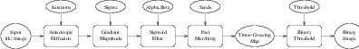
Figure 4.15 shows the major components involved in the application of the FastMarchingImageFilter to a segmentation task. It involves an initial stage of smoothing using the itk::CurvatureAnisotropicDiffusionImageFilter. The smoothed image is passed as the input to the itk::GradientMagnitudeRecursiveGaussianImageFilter and then to the itk::SigmoidImageFilter. Finally, the output of the FastMarchingImageFilter is passed to a itk::BinaryThresholdImageFilter in order to produce a binary mask representing the segmented object.
The code in the following example illustrates the typical setup of a pipeline for performing segmentation with fast marching. First, the input image is smoothed using an edge-preserving filter. Then the magnitude of its gradient is computed and passed to a sigmoid filter. The result of the sigmoid filter is the image potential that will be used to affect the speed term of the differential equation.
Let’s start by including the following headers. First we include the header of the CurvatureAnisotropicDiffusionImageFilter that will be used for removing noise from the input image.
The headers of the GradientMagnitudeRecursiveGaussianImageFilter and SigmoidImageFilter are included below. Together, these two filters will produce the image potential for regulating the speed term in the differential equation describing the evolution of the level set.
Of course, we will need the itk::Image class and the FastMarchingImageFilter class. Hence we include their headers.
The time-crossing map resulting from the FastMarchingImageFilter will be thresholded using the BinaryThresholdImageFilter. We include its header here.
Reading and writing images will be done with the itk::ImageFileReader and itk::ImageFileWriter.
We now define the image type using a pixel type and a particular dimension. In this case the float type is used for the pixels due to the requirements of the smoothing filter.
The output image, on the other hand, is declared to be binary.
The type of the BinaryThresholdImageFilter filter is instantiated below using the internal image type and the output image type.
The upper threshold passed to the BinaryThresholdImageFilter will define the time snapshot that we are taking from the time-crossing map. In an ideal application the user should be able to select this threshold interactively using visual feedback. Here, since it is a minimal example, the value is taken from the command line arguments.
We instantiate reader and writer types in the following lines.
The CurvatureAnisotropicDiffusionImageFilter type is instantiated using the internal image type.
Then, the filter is created by invoking the New() method and assigning the result to a itk::SmartPointer.
The types of the GradientMagnitudeRecursiveGaussianImageFilter and SigmoidImageFilter are instantiated using the internal image type.
The corresponding filter objects are instantiated with the New() method.
The minimum and maximum values of the SigmoidImageFilter output are defined with the methods SetOutputMinimum() and SetOutputMaximum(). In our case, we want these two values to be 0.0 and 1.0 respectively in order to get a nice speed image to feed to the FastMarchingImageFilter. Additional details on the use of the SigmoidImageFilter are presented in Section 2.3.2.
We now declare the type of the FastMarchingImageFilter.
Then, we construct one filter of this class using the New() method.
The filters are now connected in a pipeline shown in Figure 4.15 using the following lines.
The CurvatureAnisotropicDiffusionImageFilter class requires a couple of parameters to be defined. The following are typical values for 2D images. However they may have to be adjusted depending on the amount of noise present in the input image. This filter has been discussed in Section 2.7.3.
The GradientMagnitudeRecursiveGaussianImageFilter performs the equivalent of a convolution with a Gaussian kernel followed by a derivative operator. The sigma of this Gaussian can be used to control the range of influence of the image edges. This filter has been discussed in Section 2.4.2.
The SigmoidImageFilter class requires two parameters to define the linear transformation to be applied to the sigmoid argument. These parameters are passed using the SetAlpha() and SetBeta() methods. In the context of this example, the parameters are used to intensify the differences between regions of low and high values in the speed image. In an ideal case, the speed value should be 1.0 in the homogeneous regions of anatomical structures and the value should decay rapidly to 0.0 around the edges of structures. The heuristic for finding the values is the following: From the gradient magnitude image, let’s call K1 the minimum value along the contour of the anatomical structure to be segmented. Then, let’s call K2 an average value of the gradient magnitude in the middle of the structure. These two values indicate the dynamic range that we want to map to the interval [0 : 1] in the speed image. We want the sigmoid to map K1 to 0.0 and K2 to 1.0. Given that K1 is expected to be higher than K2 and we want to map those values to 0.0 and 1.0 respectively, we want to select a negative value for alpha so that the sigmoid function will also do an inverse intensity mapping. This mapping will produce a speed image such that the level set will march rapidly on the homogeneous region and will definitely stop on the contour. The suggested value for beta is (K1+K2)∕2 while the suggested value for alpha is (K2-K1)∕6, which must be a negative number. In our simple example the values are provided by the user from the command line arguments. The user can estimate these values by observing the gradient magnitude image.
The FastMarchingImageFilter requires the user to provide a seed point from which the contour will expand. The user can actually pass not only one seed point but a set of them. A good set of seed points increases the chances of segmenting a complex object without missing parts. The use of multiple seeds also helps to reduce the amount of time needed by the front to visit a whole object and hence reduces the risk of leaks on the edges of regions visited earlier. For example, when segmenting an elongated object, it is undesirable to place a single seed at one extreme of the object since the front will need a long time to propagate to the other end of the object. Placing several seeds along the axis of the object will probably be the best strategy to ensure that the entire object is captured early in the expansion of the front. One of the important properties of level sets is their natural ability to fuse several fronts implicitly without any extra bookkeeping. The use of multiple seeds takes good advantage of this property.
The seeds are passed stored in a container. The type of this container is defined as NodeContainer among the FastMarchingImageFilter traits.
Nodes are created as stack variables and initialized with a value and an itk::Index position.
The list of nodes is initialized and then every node is inserted using the InsertElement().
The set of seed nodes is now passed to the FastMarchingImageFilter with the method SetTrialPoints().
The FastMarchingImageFilter requires the user to specify the size of the image to be produced as output. This is done using the SetOutputSize() method. Note that the size is obtained here from the output image of the smoothing filter. The size of this image is valid only after the Update() method of this filter has been called directly or indirectly.
Since the front representing the contour will propagate continuously over time, it is desirable to stop the process once a certain time has been reached. This allows us to save computation time under the assumption that the region of interest has already been computed. The value for stopping the process is defined with the method SetStoppingValue(). In principle, the stopping value should be a little bit higher than the threshold value.
The invocation of the Update() method on the writer triggers the execution of the pipeline. As usual, the call is placed in a try/catch block should any errors occur or exceptions be thrown.
Now let’s run this example using the input image BrainProtonDensitySlice.png provided in the directory Examples/Data. We can easily segment the major anatomical structures by providing seeds in the appropriate locations. The following table presents the parameters used for some structures.
| Structure | Seed Index | σ | α | β | Threshold | Output Image from left | |
| Left Ventricle | (81,114) | 1.0 | -0.5 | 3.0 | 100 | First | |
| Right Ventricle | (99,114) | 1.0 | -0.5 | 3.0 | 100 | Second | |
| White matter | (56,92) | 1.0 | -0.3 | 2.0 | 200 | Third | |
| Gray matter | (40,90) | 0.5 | -0.3 | 2.0 | 200 | Fourth | |
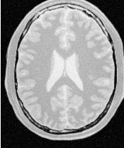
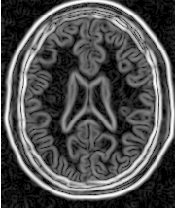
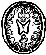
Figure 4.16 presents the intermediate outputs of the pipeline illustrated in Figure 4.15. They are from left to right: the output of the anisotropic diffusion filter, the gradient magnitude of the smoothed image and the sigmoid of the gradient magnitude which is finally used as the speed image for the FastMarchingImageFilter.


Notice that the gray matter is not being completely segmented. This illustrates the vulnerability of the level set methods when the anatomical structures to be segmented do not occupy extended regions of the image. This is especially true when the width of the structure is comparable to the size of the attenuation bands generated by the gradient filter. A possible workaround for this limitation is to use multiple seeds distributed along the elongated object. However, note that white matter versus gray matter segmentation is not a trivial task, and may require a more elaborate approach than the one used in this basic example.

The source code for this section can be found in the file
ShapeDetectionLevelSetFilter.cxx.
The use of the itk::ShapeDetectionLevelSetImageFilter is illustrated in the following example. The implementation of this filter in ITK is based on the paper by Malladi et al [38]. In this implementation, the governing differential equation has an additional curvature-based term. This term acts as a smoothing term where areas of high curvature, assumed to be due to noise, are smoothed out. Scaling parameters are used to control the tradeoff between the expansion term and the smoothing term. One consequence of this additional curvature term is that the fast marching algorithm is no longer applicable, because the contour is no longer guaranteed to always be expanding. Instead, the level set function is updated iteratively.
The ShapeDetectionLevelSetImageFilter expects two inputs, the first being an initial Level Set in the form of an itk::Image, and the second being a feature image. For this algorithm, the feature image is an edge potential image that basically follows the same rules applicable to the speed image used for the FastMarchingImageFilter discussed in Section 4.3.1.
In this example we use an FastMarchingImageFilter to produce the initial level set as the distance function to a set of user-provided seeds. The FastMarchingImageFilter is run with a constant speed value which enables us to employ this filter as a distance map calculator.
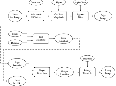
Figure 4.18 shows the major components involved in the application of the ShapeDetectionLevelSetImageFilter to a segmentation task. The first stage involves smoothing using the itk::CurvatureAnisotropicDiffusionImageFilter. The smoothed image is passed as the input for the itk::GradientMagnitudeRecursiveGaussianImageFilter and then to the itk::SigmoidImageFilter in order to produce the edge potential image. A set of user-provided seeds is passed to an FastMarchingImageFilter in order to compute the distance map. A constant value is subtracted from this map in order to obtain a level set in which the zero set represents the initial contour. This level set is also passed as input to the ShapeDetectionLevelSetImageFilter.
Finally, the level set at the output of the ShapeDetectionLevelSetImageFilter is passed to an BinaryThresholdImageFilter in order to produce a binary mask representing the segmented object.
Let’s start by including the headers of the main filters involved in the preprocessing.
The edge potential map is generated using these filters as in the previous example.
We will need the Image class, the FastMarchingImageFilter class and the ShapeDetectionLevelSetImageFilter class. Hence we include their headers here.
The level set resulting from the ShapeDetectionLevelSetImageFilter will be thresholded at the zero level in order to get a binary image representing the segmented object. The BinaryThresholdImageFilter is used for this purpose.
We now define the image type using a particular pixel type and a dimension. In this case the float type is used for the pixels due to the requirements of the smoothing filter.
The output image, on the other hand, is declared to be binary.
The type of the BinaryThresholdImageFilter filter is instantiated below using the internal image type and the output image type.
The upper threshold of the BinaryThresholdImageFilter is set to 0.0 in order to display the zero set of the resulting level set. The lower threshold is set to a large negative number in order to ensure that the interior of the segmented object will appear inside the binary region.
The CurvatureAnisotropicDiffusionImageFilter type is instantiated using the internal image type.
The filter is instantiated by invoking the New() method and assigning the result to a itk::SmartPointer.
The types of the GradientMagnitudeRecursiveGaussianImageFilter and SigmoidImageFilter are instantiated using the internal image type.
The corresponding filter objects are created with the method New().
The minimum and maximum values of the SigmoidImageFilter output are defined with the methods SetOutputMinimum() and SetOutputMaximum(). In our case, we want these two values to be 0.0 and 1.0 respectively in order to get a nice speed image to feed to the FastMarchingImageFilter. Additional details on the use of the SigmoidImageFilter are presented in Section 2.3.2.
We now declare the type of the FastMarchingImageFilter that will be used to generate the initial level set in the form of a distance map.
Next we construct one filter of this class using the New() method.
In the following lines we instantiate the type of the ShapeDetectionLevelSetImageFilter and create an object of this type using the New() method.
The filters are now connected in a pipeline indicated in Figure 4.18 with the following code.
smoothing->SetInput( reader->GetOutput() );
gradientMagnitude->SetInput( smoothing->GetOutput() );
sigmoid->SetInput( gradientMagnitude->GetOutput() );
shapeDetection->SetInput( fastMarching->GetOutput() );
shapeDetection->SetFeatureImage( sigmoid->GetOutput() );
thresholder->SetInput( shapeDetection->GetOutput() );
writer->SetInput( thresholder->GetOutput() );
The CurvatureAnisotropicDiffusionImageFilter requires a couple of parameters to be defined. The following are typical values for 2D images. However they may have to be adjusted depending on the amount of noise present in the input image. This filter has been discussed in Section 2.7.3.
The GradientMagnitudeRecursiveGaussianImageFilter performs the equivalent of a convolution with a Gaussian kernel followed by a derivative operator. The sigma of this Gaussian can be used to control the range of influence of the image edges. This filter has been discussed in Section 2.4.2.
The SigmoidImageFilter requires two parameters that define the linear transformation to be applied to the sigmoid argument. These parameters have been discussed in Sections 2.3.2 and 4.3.1.
The FastMarchingImageFilter requires the user to provide a seed point from which the level set will be generated. The user can actually pass not only one seed point but a set of them. Note the FastMarchingImageFilter is used here only as a helper in the determination of an initial level set. We could have used the itk::DanielssonDistanceMapImageFilter in the same way.
The seeds are stored in a container. The type of this container is defined as NodeContainer among the FastMarchingImageFilter traits.
Nodes are created as stack variables and initialized with a value and an itk::Index position. Note that we assign the negative of the value of the user-provided distance to the unique node of the seeds passed to the FastMarchingImageFilter. In this way, the value will increment as the front is propagated, until it reaches the zero value corresponding to the contour. After this, the front will continue propagating until it fills up the entire image. The initial distance is taken from the command line arguments. The rule of thumb for the user is to select this value as the distance from the seed points at which the initial contour should be.
The list of nodes is initialized and then every node is inserted using InsertElement().
The set of seed nodes is now passed to the FastMarchingImageFilter with the method SetTrialPoints().
Since the FastMarchingImageFilter is used here only as a distance map generator, it does not require a speed image as input. Instead, the constant value 1.0 is passed using the SetSpeedConstant() method.
The FastMarchingImageFilter requires the user to specify the size of the image to be produced as output. This is done using the SetOutputSize(). Note that the size is obtained here from the output image of the smoothing filter. The size of this image is valid only after the Update() methods of this filter have been called directly or indirectly.
ShapeDetectionLevelSetImageFilter provides two parameters to control the competition between the propagation or expansion term and the curvature smoothing term. The methods SetPropagationScaling() and SetCurvatureScaling() defines the relative weighting between the two terms. In this example, we will set the propagation scaling to one and let the curvature scaling be an input argument. The larger the the curvature scaling parameter the smoother the resulting segmentation. However, the curvature scaling parameter should not be set too large, as it will draw the contour away from the shape boundaries.
Once activated, the level set evolution will stop if the convergence criteria or the maximum number of iterations is reached. The convergence criteria are defined in terms of the root mean squared (RMS) change in the level set function. The evolution is said to have converged if the RMS change is below a user-specified threshold. In a real application, it is desirable to couple the evolution of the zero set to a visualization module, allowing the user to follow the evolution of the zero set. With this feedback, the user may decide when to stop the algorithm before the zero set leaks through the regions of low gradient in the contour of the anatomical structure to be segmented.
The invocation of the Update() method on the writer triggers the execution of the pipeline. As usual, the call is placed in a try/catch block should any errors occur or exceptions be thrown.
Let’s now run this example using as input the image BrainProtonDensitySlice.png provided in the directory Examples/Data. We can easily segment the major anatomical structures by providing seeds in the appropriate locations. Table 4.4 presents the parameters used for some structures. For all of the examples illustrated in this table, the propagation scaling was set to 1.0, and the curvature scaling set to 0.05.
Figure 4.19 presents the intermediate outputs of the pipeline illustrated in Figure 4.18. They are from left to right: the output of the anisotropic diffusion filter, the gradient magnitude of the smoothed image and the sigmoid of the gradient magnitude which is finally used as the edge potential for the ShapeDetectionLevelSetImageFilter.
Notice that in Figure 4.20 the segmented shapes are rounder than in Figure 4.17 due to the effects of the curvature term in the driving equation. As with the previous example, segmentation of the gray matter is still problematic.

A larger number of iterations is reguired for segmenting large structures since it takes longer for the front to propagate and cover the structure. This drawback can be easily mitigated by setting many seed points in the initialization of the FastMarchingImageFilter. This will generate an initial level set much closer in shape to the object to be segmented and hence require fewer iterations to fill and reach the edges of the anatomical structure.


The source code for this section can be found in the file
GeodesicActiveContourImageFilter.cxx.
The use of the itk::GeodesicActiveContourLevelSetImageFilter is illustrated in the following example. The implementation of this filter in ITK is based on the paper by Caselles [11]. This implementation extends the functionality of the itk::ShapeDetectionLevelSetImageFilter by the addition of a third advection term which attracts the level set to the object boundaries.
GeodesicActiveContourLevelSetImageFilter expects two inputs. The first is an initial level set in the form of an itk::Image. The second input is a feature image. For this algorithm, the feature image is an edge potential image that basically follows the same rules used for the ShapeDetectionLevelSetImageFilter discussed in Section 4.3.2. The configuration of this example is quite similar to the example on the use of the ShapeDetectionLevelSetImageFilter. We omit most of the redundant description. A look at the code will reveal the great degree of similarity between both examples.
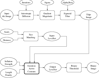
Figure 4.21 shows the major components involved in the application of the GeodesicActiveContourLevelSetImageFilter to a segmentation task. This pipeline is quite similar to the one used by the ShapeDetectionLevelSetImageFilter in section 4.3.2.
The pipeline involves a first stage of smoothing using the
itk::CurvatureAnisotropicDiffusionImageFilter. The smoothed image is passed as the
input to the itk::GradientMagnitudeRecursiveGaussianImageFilter and then to the
itk::SigmoidImageFilter in order to produce the edge potential image. A set of user-provided seeds is
passed to a itk::FastMarchingImageFilter in order to compute the distance map. A constant value is
subtracted from this map in order to obtain a level set in which the zero set represents the initial contour.
This level set is also passed as input to the GeodesicActiveContourLevelSetImageFilter.
Finally, the level set generated by the GeodesicActiveContourLevelSetImageFilter is passed to a itk::BinaryThresholdImageFilter in order to produce a binary mask representing the segmented object.
Let’s start by including the headers of the main filters involved in the preprocessing.
We now define the image type using a particular pixel type and dimension. In this case the float type is used for the pixels due to the requirements of the smoothing filter.
In the following lines we instantiate the type of the GeodesicActiveContourLevelSetImageFilter and create an object of this type using the New() method.
For the GeodesicActiveContourLevelSetImageFilter, scaling parameters are used to trade off between the propagation (inflation), the curvature (smoothing) and the advection terms. These parameters are set using methods SetPropagationScaling(), SetCurvatureScaling() and SetAdvectionScaling(). In this example, we will set the curvature and advection scales to one and let the propagation scale be a command-line argument.
The filters are now connected in a pipeline indicated in Figure 4.21 using the following lines:
smoothing->SetInput( reader->GetOutput() );
gradientMagnitude->SetInput( smoothing->GetOutput() );
sigmoid->SetInput( gradientMagnitude->GetOutput() );
geodesicActiveContour->SetInput( fastMarching->GetOutput() );
geodesicActiveContour->SetFeatureImage( sigmoid->GetOutput() );
thresholder->SetInput( geodesicActiveContour->GetOutput() );
writer->SetInput( thresholder->GetOutput() );
The invocation of the Update() method on the writer triggers the execution of the pipeline. As usual, the call is placed in a try/catch block should any errors occur or exceptions be thrown.
Let’s now run this example using as input the image BrainProtonDensitySlice.png provided in the directory Examples/Data. We can easily segment the major anatomical structures by providing seeds in the appropriate locations. Table 4.5 presents the parameters used for some structures.
| Structure | Seed Index | Distance | σ | α | β | Propag. | Output Image | |
| Left Ventricle | (81,114) | 5.0 | 1.0 | -0.5 | 3.0 | 2.0 | First | |
| Right Ventricle | (99,114) | 5.0 | 1.0 | -0.5 | 3.0 | 2.0 | Second | |
| White matter | (56,92) | 5.0 | 1.0 | -0.3 | 2.0 | 10.0 | Third | |
| Gray matter | (40,90) | 5.0 | 0.5 | -0.3 | 2.0 | 10.0 | Fourth | |
Figure 4.22 presents the intermediate outputs of the pipeline illustrated in Figure 4.21. They are from left to right: the output of the anisotropic diffusion filter, the gradient magnitude of the smoothed image and the sigmoid of the gradient magnitude which is finally used as the edge potential for the GeodesicActiveContourLevelSetImageFilter.

Segmentations of the main brain structures are presented in Figure 4.23. The results are quite similar to those obtained with the ShapeDetectionLevelSetImageFilter in Section 4.3.2.
Note that a relatively larger propagation scaling value was required to segment the white matter. This is due to two factors: the lower contrast at the border of the white matter and the complex shape of the structure. Unfortunately the optimal value of these scaling parameters can only be determined by experimentation. In a real application we could imagine an interactive mechanism by which a user supervises the contour evolution and adjusts these parameters accordingly.


The source code for this section can be found in the file
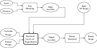
ThresholdSegmentationLevelSetImageFilter.cxx.
The itk::ThresholdSegmentationLevelSetImageFilter is an extension of the threshold connected-component segmentation to the level set framework. The goal is to define a range of intensity values that classify the tissue type of interest and then base the propagation term on the level set equation for that intensity range. Using the level set approach, the smoothness of the evolving surface can be constrained to prevent some of the “leaking” that is common in connected-component schemes.
The propagation term P from Equation 4.3 is calculated from the FeatureImage input g with UpperThreshold U and LowerThreshold L according to the following formula.
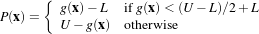 | (4.4) |
Figure 4.25 illustrates the propagation term function. Intensity values in g between L and H yield positive values in P, while outside intensities yield negative values in P.
The threshold segmentation filter expects two inputs. The first is an initial level set in the form of an itk::Image. The second input is the feature image g. For many applications, this filter requires little or no preprocessing of its input. Smoothing the input image is not usually required to produce reasonable solutions, though it may still be warranted in some cases.
Figure 4.24 shows how the image processing pipeline is constructed. The initial surface is generated using the fast marching filter. The output of the segmentation filter is passed to a itk::BinaryThresholdImageFilter to create a binary representation of the segmented object. Let’s start by including the appropriate header file.
We define the image type using a particular pixel type and dimension. In this case we will use 2D float images.
The following lines instantiate a ThresholdSegmentationLevelSetImageFilter using the New() method.
For the ThresholdSegmentationLevelSetImageFilter, scaling parameters are used to balance the influence of the propagation (inflation) and the curvature (surface smoothing) terms from Equation 4.3. The advection term is not used in this filter. Set the terms with methods SetPropagationScaling() and SetCurvatureScaling(). Both terms are set to 1.0 in this example.
The convergence criteria MaximumRMSError and MaximumIterations are set as in previous examples. We now set the upper and lower threshold values U and L, and the isosurface value to use in the initial model.
The filters are now connected in a pipeline indicated in Figure 4.24. Remember that before calling Update() on the file writer object, the fast marching filter must be initialized with the seed points and the output from the reader object. See previous examples and the source code for this section for details.
Invoking the Update() method on the writer triggers the execution of the pipeline. As usual, the call is placed in a try/catch block should any errors occur or exceptions be thrown.
try
{
reader->Update();
const InternalImageType ⋆ inputImage = reader->GetOutput();
fastMarching->SetOutputRegion( inputImage->GetBufferedRegion() );
fastMarching->SetOutputSpacing( inputImage->GetSpacing() );
fastMarching->SetOutputOrigin( inputImage->GetOrigin() );
fastMarching->SetOutputDirection( inputImage->GetDirection() );
writer->Update();
}
catch( itk::ExceptionObject & excep )
{
std::cerr << "Exception caught !" << std::endl;
std::cerr << excep << std::endl;
return EXIT_FAILURE;
}
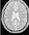
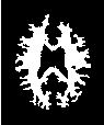
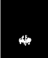
Let’s run this application with the same data and parameters as the example given for itk::ConnectedThresholdImageFilter in Section 4.1.1. We will use a value of 5 as the initial distance of the surface from the seed points. The algorithm is relatively insensitive to this initialization. Compare the results in Figure 4.26 with those in Figure 4.1. Notice how the smoothness constraint on the surface prevents leakage of the segmentation into both ventricles, but also localizes the segmentation to a smaller portion of the gray matter.

| Structure | Seed Index | Lower | Upper | Output Image | |
| White matter | (60,116) | 150 | 180 | Second from left | |
| Ventricle | (81,112) | 210 | 250 | Third from left | |
| Gray matter | (107,69) | 180 | 210 | Fourth from left | |
The source code for this section can be found in the file
CannySegmentationLevelSetImageFilter.cxx.
The itk::CannySegmentationLevelSetImageFilter defines a speed term that minimizes distance to the Canny edges in an image. The initial level set model moves through a gradient advection field until it locks onto those edges. This filter is more suitable for refining existing segmentations than as a region-growing algorithm.
The two terms defined for the CannySegmentationLevelSetImageFilter are the advection term and the propagation term from Equation 4.3. The advection term is constructed by minimizing the squared distance transform from the Canny edges.
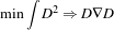 | (4.5) |
where the distance transform D is calculated using a itk::DanielssonDistanceMapImageFilter applied to the output of the itk::CannyEdgeDetectionImageFilter.
For cases in which some surface expansion is to be allowed, a non-zero value may be set for the propagation term. The propagation term is simply D. As with all ITK level set segmentation filters, the curvature term controls the smoothness of the surface.
CannySegmentationLevelSetImageFilter expects two inputs. The first is an initial level set in the form of an itk::Image. The second input is the feature image g from which propagation and advection terms are calculated. It is generally a good idea to do some preprocessing of the feature image to remove noise.
Figure 4.27 shows how the image processing pipeline is constructed. We read two images: the image to segment and the image that contains the initial implicit surface. The goal is to refine the initial model from the second input and not to grow a new segmentation from seed points. The feature image is preprocessed with a few iterations of an anisotropic diffusion filter.
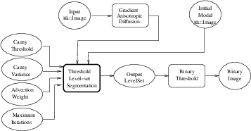
Let’s start by including the appropriate header file.
We define the image type using a particular pixel type and dimension. In this case we will use 2D float images.
The input image will be processed with a few iterations of feature-preserving diffusion. We create a filter and set the appropriate parameters.
The following lines define and instantiate a CannySegmentationLevelSetImageFilter.
As with the other ITK level set segmentation filters, the terms of the CannySegmentationLevelSetImageFilter level set equation can be weighted by scalars. For this application we will modify the relative weight of the advection term. The propagation and curvature term weights are set to their defaults of 0 and 1, respectively.
The maximum number of iterations is specified from the command line. It may not be desirable in some applications to run the filter to convergence. Only a few iterations may be required.
There are two important parameters in the CannySegmentationLevelSetImageFilter to control the behavior of the Canny edge detection. The variance parameter controls the amount of Gaussian smoothing on the input image. The threshold parameter indicates the lowest allowed value in the output image. Thresholding is used to suppress Canny edges whose gradient magnitudes fall below a certain value.
Finally, it is very important to specify the isovalue of the surface in the initial model input image. In a binary image, for example, the isosurface is found midway between the foreground and background values.
The filters are now connected in a pipeline indicated in Figure 4.27.
Invoking the Update() method on the writer triggers the execution of the pipeline. As usual, the call is placed in a try/catch block to handle any exceptions that may be thrown.
We can use this filter to make some subtle refinements to the ventricle segmentation from the previous example that used the itk::ThresholdSegmentationLevelSetImageFilter. The application was run using Examples/Data/BrainProtonDensitySlice.png and Examples/Data/VentricleModel.png as inputs, a threshold of 7.0, variance of 0.1, advection weight of 10.0, and an initial isosurface value of 127.5. One case was run for 15 iterations and the second was run to convergence. Compare the results in the two rightmost images of Figure 4.28 with the ventricle segmentation from Figure 4.26 shown in the middle. Jagged edges are straightened and the small spur at the upper right-hand side of the mask has been removed.


The free parameters of this filter can be adjusted to achieve a wide range of shape variations from the original model. Finding the right parameters for your particular application is usually a process of trial and error. As with most ITK level set segmentation filters, examining the propagation (speed) and advection images can help the process of tuning parameters. These images are available using Set/Get methods from the filter after it has been updated.
In some cases it is interesting to take a direct look at the speed image used internally by this filter. This may help for setting the correct parameters for driving the segmentation. In order to obtain such speed image, the method GenerateSpeedImage() should be invoked first. Then we can recover the speed image with the GetSpeedImage() method as illustrated in the following lines.
cannySegmentation->GenerateSpeedImage();
using SpeedImageType =
CannySegmentationLevelSetImageFilterType::SpeedImageType;
using SpeedWriterType = itk::ImageFileWriter<SpeedImageType>;
SpeedWriterType::Pointer speedWriter = SpeedWriterType::New();
speedWriter->SetInput( cannySegmentation->GetSpeedImage() );
The source code for this section can be found in the file
LaplacianSegmentationLevelSetImageFilter.cxx.
The itk::LaplacianSegmentationLevelSetImageFilter defines a speed term based on second derivative features in the image. The speed term is calculated as the Laplacian of the image values. The goal is to attract the evolving level set surface to local zero-crossings in the Laplacian image. Like itk::CannySegmentationLevelSetImageFilter, this filter is more suitable for refining existing segmentations than as a stand-alone, region growing algorithm. It is possible to perform region growing segmentation, but be aware that the growing surface may tend to become “stuck” at local edges.
The propagation (speed) term for the LaplacianSegmentationLevelSetImageFilter is constructed by applying the itk::LaplacianImageFilter to the input feature image. One nice property of using the Laplacian is that there are no free parameters in the calculation.
LaplacianSegmentationLevelSetImageFilter expects two inputs. The first is an initial level set in the form of an itk::Image. The second input is the feature image g from which the propagation term is calculated (see Equation 4.3). Because the filter performs a second derivative calculation, it is generally a good idea to do some preprocessing of the feature image to remove noise.
Figure 4.29 shows how the image processing pipeline is constructed. We read two images: the image to segment and the image that contains the initial implicit surface. The goal is to refine the initial model from the second input to better match the structure represented by the initial implicit surface (a prior segmentation). The feature image is preprocessed using an anisotropic diffusion filter.
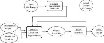
Let’s start by including the appropriate header files.
We define the image type using a particular pixel type and dimension. In this case we will use 2D float images.
The input image will be processed with a few iterations of feature-preserving diffusion. We create a filter and set the parameters. The number of iterations and the conductance parameter are taken from the command line.
using DiffusionFilterType =
itk::GradientAnisotropicDiffusionImageFilter< InternalImageType,
InternalImageType >;
DiffusionFilterType::Pointer diffusion = DiffusionFilterType::New();
diffusion->SetNumberOfIterations( std::stoi(argv[4]) );
diffusion->SetTimeStep(0.125);
diffusion->SetConductanceParameter( std::stod(argv[5]) );
The following lines define and instantiate a LaplacianSegmentationLevelSetImageFilter.
As with the other ITK level set segmentation filters, the terms of the LaplacianSegmentationLevelSetImageFilter level set equation can be weighted by scalars. For this application we will modify the relative weight of the propagation term. The curvature term weight is set to its default of 1. The advection term is not used in this filter.
The maximum number of iterations is set from the command line. It may not be desirable in some applications to run the filter to convergence. Only a few iterations may be required.
Finally, it is very important to specify the isovalue of the surface in the initial model input image. In a binary image, for example, the isosurface is found midway between the foreground and background values.
The filters are now connected in a pipeline indicated in Figure 4.29.
Invoking the Update() method on the writer triggers the execution of the pipeline. As usual, the call is placed in a try/catch block to handle any exceptions that may be thrown.
We can use this filter to make some subtle refinements to the ventricle segmentation from the example using the filter itk::ThresholdSegmentationLevelSetImageFilter. This application was run using Examples/Data/BrainProtonDensitySlice.png and Examples/Data/VentricleModel.png as inputs. We used 10 iterations of the diffusion filter with a conductance of 2.0. The propagation scaling was set to 1.0 and the filter was run until convergence. Compare the results in the rightmost images of Figure 4.30 with the ventricle segmentation from Figure 4.26 shown in the middle. Jagged edges are straightened and the small spur at the upper right-hand side of the mask has been removed.

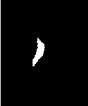

The source code for this section can be found in the file
GeodesicActiveContourShapePriorLevelSetImageFilter.cxx.
In medical imaging applications, the general shape, location and orientation of an anatomical structure of interest is typically known a priori. This information can be used to aid the segmentation process especially when image contrast is low or when the object boundary is not distinct.
In [33], Leventon et al. extended the geodesic active contours method with an additional shape-influenced term in the driving PDE. The itk::GeodesicActiveContourShapePriorLevelSetFilter is a generalization of Leventon’s approach and its use is illustrated in the following example.
To support shape-guidance, the generic level set equation (Eqn( 4.3)) is extended to incorporate a shape guidance term:
 | (4.6) |
where ψ* is the signed distance function of the “best-fit” shape with respect to a shape model. The new term has the effect of driving the contour towards the best-fit shape. The scalar ξ weights the influence of the shape term in the overall evolution. In general, the best-fit shape is not known ahead of time and has to be iteratively estimated in conjunction with the contour evolution.
As with the itk::GeodesicActiveContourLevelSetImageFilter, the GeodesicActiveContourShapePriorLevelSetImageFilter expects two input images: the first is an initial level set and the second a feature image that represents the image edge potential. The configuration of this example is quite similar to the example in Section 4.3.3 and hence the description will focus on the new objects involved in the segmentation process as shown in Figure 4.31.
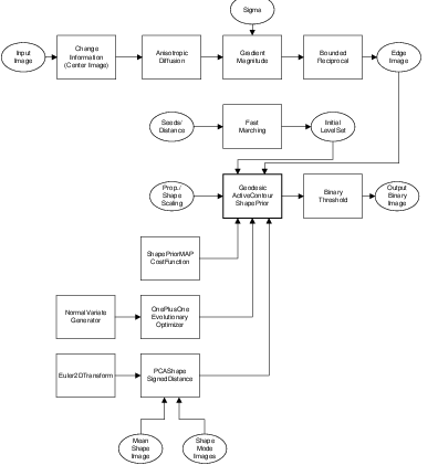
The process pipeline begins with centering the input image using the the itk::ChangeInformationImageFilter to simplify the estimation of the pose of the shape, to be explained later. The centered image is then smoothed using non-linear diffusion to remove noise and the gradient magnitude is computed from the smoothed image. For simplicity, this example uses the itk::BoundedReciprocalImageFilter to produce the edge potential image.
The itk::FastMarchingImageFilter creates an initial level set using three user specified seed positions and a initial contour radius. Three seeds are used in this example to facilitate the segmentation of long narrow objects in a smaller number of iterations. The output of the FastMarchingImageFilter is passed as the input to the GeodesicActiveContourShapePriorLevelSetImageFilter. At then end of the segmentation process, the output level set is passed to the itk::BinaryThresholdImageFilter to produce a binary mask representing the segmented object.
The remaining objects in Figure 4.31 are used for shape modeling and estimation. The itk::PCAShapeSignedDistanceFunction represents a statistical shape model defined by a mean signed distance and the first K principal components modes; while the itk::Euler2DTransform is used to represent the pose of the shape. In this implementation, the best-fit shape estimation problem is reformulated as a minimization problem where the itk::ShapePriorMAPCostFunction is the cost function to be optimized using the itk::OnePlusOneEvolutionaryOptimizer.
It should be noted that, although particular shape model, transform cost function, and optimizer are used in this example, the implementation is generic, allowing different instances of these components to be plugged in. This flexibility allows a user to tailor the behavior of the segmentation process to suit the circumstances of the targeted application.
Let’s start the example by including the headers of the new filters involved in the segmentation.
Next, we include the headers of the objects involved in shape modeling and estimation.
Given the numerous parameters involved in tuning this segmentation method it is not uncommon for a segmentation process to run for several minutes and still produce an unsatisfactory result. For debugging purposes it is quite helpful to track the evolution of the segmentation as it progresses. The following defines a custom itk::Command class for monitoring the RMS change and shape parameters at each iteration.
#include "itkCommand.h"
template<class TFilter>
class CommandIterationUpdate : public itk::Command
{
public:
using Self = CommandIterationUpdate;
using Superclass = itk::Command;
using Pointer = itk::SmartPointer<Self>;
itkNewMacro( Self );
protected:
CommandIterationUpdate() = default;
public:
void Execute(itk::Object ⋆caller,
const itk::EventObject & event) override
{
Execute( (const itk::Object ⋆) caller, event);
}
void Execute(const itk::Object ⋆ object,
const itk::EventObject & event) override
{
const auto ⋆ filter = static_cast< const TFilter ⋆ >( object );
if( typeid( event ) != typeid( itk::IterationEvent ) )
{ return; }
std::cout << filter->GetElapsedIterations() << ": ";
std::cout << filter->GetRMSChange() << " ";
std::cout << filter->GetCurrentParameters() << std::endl;
}
};
We define the image type using a particular pixel type and dimension. In this case we will use 2D float images.
The following line instantiate a itk::GeodesicActiveContourShapePriorLevelSetImageFilter using the New() method.
The itk::ChangeInformationImageFilter is the first filter in the preprocessing stage and is used to force the image origin to the center of the image.
In this example, we will use the bounded reciprocal 1∕(1+x) of the image gradient magnitude as the edge potential feature image.
In the GeodesicActiveContourShapePriorLevelSetImageFilter, scaling parameters are used to trade off between the propagation (inflation), the curvature (smoothing), the advection, and the shape influence terms. These parameters are set using methods SetPropagationScaling(), SetCurvatureScaling(), SetAdvectionScaling() and SetShapePriorScaling(). In this example, we will set the curvature and advection scales to one and let the propagation and shape prior scale be command-line arguments.
Each iteration, the current “best-fit” shape is estimated from the edge potential image and the current contour. To increase speed, only information within the sparse field layers of the current contour is used in the estimation. The default number of sparse field layers is the same as the ImageDimension which does not contain enough information to get a reliable best-fit shape estimate. Thus, we override the default and set the number of layers to 4.
The filters are then connected in a pipeline as illustrated in Figure 4.31.
center->SetInput( reader->GetOutput() );
smoothing->SetInput( center->GetOutput() );
gradientMagnitude->SetInput( smoothing->GetOutput() );
reciprocal->SetInput( gradientMagnitude->GetOutput() );
geodesicActiveContour->SetInput( fastMarching->GetOutput() );
geodesicActiveContour->SetFeatureImage( reciprocal->GetOutput() );
thresholder->SetInput( geodesicActiveContour->GetOutput() );
writer->SetInput( thresholder->GetOutput() );
Next, we define the shape model. In this example, we use an implicit shape model based on the principal components such that:
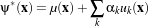 | (4.7) |
where μ(x) is the mean signed distance computed from training set of segmented objects and uk(x) are the first K principal components of the offset (signed distance - mean). The coefficients {αk} form the set of shape parameters.
Given a set of training data, the itk::ImagePCAShapeModelEstimator can be used to obtain the mean and principal mode shape images required by PCAShapeSignedDistanceFunction.
In this example, we will read the mean shape and principal mode images from file. We will assume that the filenames of the mode images form a numeric series starting from index 0.
ReaderType::Pointer meanShapeReader = ReaderType::New();
meanShapeReader->SetFileName( argv[13] );
meanShapeReader->Update();
std::vector<InternalImageType::Pointer> shapeModeImages( numberOfPCAModes );
itk::NumericSeriesFileNames::Pointer fileNamesCreator =
itk::NumericSeriesFileNames::New();
fileNamesCreator->SetStartIndex( 0 );
fileNamesCreator->SetEndIndex( numberOfPCAModes - 1 );
fileNamesCreator->SetSeriesFormat( argv[15] );
const std::vector<std::string> & shapeModeFileNames =
fileNamesCreator->GetFileNames();
for (unsigned int k = 0; k < numberOfPCAModes; ++k )
{
ReaderType::Pointer shapeModeReader = ReaderType::New();
shapeModeReader->SetFileName( shapeModeFileNames[k].c_str() );
shapeModeReader->Update();
shapeModeImages[k] = shapeModeReader->GetOutput();
}
shape->SetMeanImage( meanShapeReader->GetOutput() );
shape->SetPrincipalComponentImages( shapeModeImages );
Further we assume that the shape modes have been normalized by multiplying with the corresponding singular value. Hence, we can set the principal component standard deviations to all ones.
Next, we instantiate a itk::Euler2DTransform and connect it to the PCASignedDistanceFunction. The transform represent the pose of the shape. The parameters of the transform forms the set of pose parameters.
Before updating the level set at each iteration, the parameters of the current best-fit shape is estimated by minimizing the itk::ShapePriorMAPCostFunction. The cost function is composed of four terms: contour fit, image fit, shape prior and pose prior. The user can specify the weights applied to each term.
using CostFunctionType = itk::ShapePriorMAPCostFunction<
InternalImageType,
InternalPixelType >;
CostFunctionType::Pointer costFunction = CostFunctionType::New();
CostFunctionType::WeightsType weights;
weights[0] = 1.0; // weight for contour fit term
weights[1] = 20.0; // weight for image fit term
weights[2] = 1.0; // weight for shape prior term
weights[3] = 1.0; // weight for pose prior term
costFunction->SetWeights( weights );
Contour fit measures the likelihood of seeing the current evolving contour for a given set of shape/pose parameters. This is computed by counting the number of pixels inside the current contour but outside the current shape.
Image fit measures the likelihood of seeing certain image features for a given set of shape/pose parameters. This is computed by assuming that ( 1 - edge potential ) approximates a zero-mean, unit variance Gaussian along the normal of the evolving contour. Image fit is then computed by computing the Laplacian goodness of fit of the Gaussian:
 | (4.8) |
where G is a zero-mean, unit variance Gaussian and g is the edge potential feature image.
The pose parameters are assumed to have a uniform distribution and hence do not contribute to the cost function. The shape parameters are assumed to have a Gaussian distribution. The parameters of the distribution are user-specified. Since we assumed the principal modes have already been normalized, we set the distribution to zero mean and unit variance.
In this example, we will use the itk::OnePlusOneEvolutionaryOptimizer to optimize the cost function.
The evolutionary optimization algorithm is based on testing random permutations of the parameters. As such, we need to provide the optimizer with a random number generator. In the following lines, we create a itk::NormalVariateGenerator, seed it, and connect it to the optimizer.
The cost function has K +3 parameters. The first K parameters are the principal component multipliers, followed by the 2D rotation parameter (in radians) and the x- and y- translation parameters (in mm). We need to carefully scale the different types of parameters to compensate for the differences in the dynamic ranges of the parameters.
Next, we specify the initial radius, the shrink and grow mutation factors and termination criteria of the optimizer. Since the best-fit shape is re-estimated each iteration of the curve evolution, we do not need to spend too much time finding the true minimizing solution each time; we only need to head towards it. As such, we only require a small number of optimizer iterations.
Before starting the segmentation process we need to also supply the initial best-fit shape estimate. In this example, we start with the unrotated mean shape with the initial x- and y- translation specified through command-line arguments.
Finally, we connect all the components to the filter and add our observer.
geodesicActiveContour->SetShapeFunction( shape );
geodesicActiveContour->SetCostFunction( costFunction );
geodesicActiveContour->SetOptimizer( optimizer );
geodesicActiveContour->SetInitialParameters( parameters );
using CommandType = CommandIterationUpdate<GeodesicActiveContourFilterType>;
CommandType::Pointer observer = CommandType::New();
geodesicActiveContour->AddObserver( itk::IterationEvent(), observer );
The invocation of the Update() method on the writer triggers the execution of the pipeline. As usual, the call is placed in a try/catch block to handle exceptions should errors occur.
Deviating from previous examples, we will demonstrate this example using BrainMidSagittalSlice.png (Figure 4.32, left) from the Examples/Data directory. The aim here is to segment the corpus callosum from the image using a shape model defined by CorpusCallosumMeanShape.mha and the first three principal components CorpusCallosumMode0.mha, CorpusCallosumMode1.mha and CorpusCallosumMode12.mha. As shown in Figure 4.33, the first mode captures scaling, the second mode captures the shifting of mass between the rostrum and the splenium and the third mode captures the degree of curvature. Segmentation results with and without shape guidance are shown in Figure 4.34.
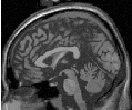

| -3σ | mean | +3σ | |
| mode 0: |  |  |  |
| mode 1: |  |  |  |
| mode 2: |  |  |  |
A sigma value of 1.0 was used to compute the image gradient and the propagation and shape prior scaling are respectively set to 0.5 and 0.02. An initial level set was created by placing one seed point in the rostrum (60,102), one in the splenium (120,85) and one centrally in the body (88,83) of the corpus callosum with an initial radius of 6 pixels at each seed position. The best-fit shape was initially placed with a translation of (10,0)mm so that it roughly overlapped the corpus callosum in the image as shown in Figure 4.32 (right).
From Figure 4.34 it can be observed that without shape guidance (left), segmentation using geodesic active contour leaks in the regions where the corpus callosum blends into the surrounding brain tissues. With shape guidance (center), the segmentation is constrained by the global shape model to prevent leaking.
The final best-fit shape parameters after the segmentation process is:
and is shown in Figure 4.34 (right). Note that a 0.28 radian (15.8 degree) rotation has been introduced to match the model to the corpus callosum in the image. Additionally, a negative weight for the first mode shrinks the size relative to the mean shape. A negative weight for the second mode shifts the mass to splenium, and a positive weight for the third mode increases the curvature. It can also be observed that the final segmentation is a combination of the best-fit shape with additional local deformation. The combination of both global and local shape allows the segmentation to capture fine details not represented in the shape model.


Extracting salient features from images is an important task on image processing. It is typically used for guiding segmentation methods, preparing data for registration methods, or as a mechanism for recognizing anatomical structures in images. The following section introduce some of the feature extraction methods available in ITK.
The Hough transform is a widely used technique for detection of geometrical features in images. It is based on mapping the image into a parametric space in which it may be easier to identify if particular geometrical features are present in the image. The transformation is specific for each desired geometrical shape.
The source code for this section can be found in the file
HoughTransform2DLinesImageFilter.cxx.
This example illustrates the use of the itk::HoughTransform2DLinesImageFilter to find straight lines in a 2-dimensional image.
First, we include the header files of the filter.
Next, we declare the pixel type and image dimension and specify the image type to be used as input. We also specify the image type of the accumulator used in the Hough transform filter.
We setup a reader to load the input image.
using ReaderType = itk::ImageFileReader< ImageType >;
ReaderType::Pointer reader = ReaderType::New();
reader->SetFileName( argv[1] );
try
{
reader->Update();
}
catch( itk::ExceptionObject & excep )
{
std::cerr << "Exception caught !" << std::endl;
std::cerr << excep << std::endl;
return EXIT_FAILURE;
}
ImageType::Pointer localImage = reader->GetOutput();
Once the image is loaded, we apply a itk::GradientMagnitudeImageFilter to segment edges. This casts the input image using a itk::CastImageFilter.
using CastingFilterType =
itk::CastImageFilter< ImageType, AccumulatorImageType >;
CastingFilterType::Pointer caster = CastingFilterType::New();
std::cout << "Applying gradient magnitude filter" << std::endl;
using GradientFilterType =
itk::GradientMagnitudeImageFilter< AccumulatorImageType,
AccumulatorImageType >;
GradientFilterType::Pointer gradFilter = GradientFilterType::New();
caster->SetInput(localImage);
gradFilter->SetInput(caster->GetOutput());
gradFilter->Update();
The next step is to apply a threshold filter on the gradient magnitude image to keep only bright values. Only pixels with a high value will be used by the Hough transform filter.
std::cout << "Thresholding" << std::endl;
using ThresholdFilterType = itk::ThresholdImageFilter<AccumulatorImageType>;
ThresholdFilterType::Pointer threshFilter = ThresholdFilterType::New();
threshFilter->SetInput( gradFilter->GetOutput());
threshFilter->SetOutsideValue(0);
unsigned char threshBelow = 0;
unsigned char threshAbove = 255;
threshFilter->ThresholdOutside(threshBelow,threshAbove);
threshFilter->Update();
We create the HoughTransform2DLinesImageFilter based on the pixel type of the input image (the resulting image from the ThresholdImageFilter).
We set the input to the filter to be the output of the ThresholdImageFilter. We set also the number of lines we are looking for. Basically, the filter computes the Hough map, blurs it using a certain variance and finds maxima in the Hough map. After a maximum is found, the local neighborhood, a circle, is removed from the Hough map. SetDiscRadius() defines the radius of this disc.
The output of the filter is the accumulator.
houghFilter->SetInput(threshFilter->GetOutput());
houghFilter->SetNumberOfLines(std::stoi(argv[3]));
if(argc > 4 )
{
houghFilter->SetVariance(std::stod(argv[4]));
}
if(argc > 5 )
{
houghFilter->SetDiscRadius(std::stod(argv[5]));
}
houghFilter->Update();
AccumulatorImageType::Pointer localAccumulator = houghFilter->GetOutput();
We can also get the lines as itk::LineSpatialObject. The GetLines() function return a list of those.
We can then allocate an image to draw the resulting lines as binary objects.
using OutputPixelType = unsigned char;
using OutputImageType = itk::Image< OutputPixelType, Dimension >;
OutputImageType::Pointer localOutputImage = OutputImageType::New();
OutputImageType::RegionType region(localImage->GetLargestPossibleRegion());
localOutputImage->SetRegions(region);
localOutputImage->CopyInformation(localImage);
localOutputImage->Allocate(true); // initialize buffer to zero
We iterate through the list of lines and we draw them.
We get the list of points which consists of two points to represent a straight line. Then, from these two
points, we compute a fixed point u and a unit vector  to parameterize the line.
using LinePointListType =
HoughTransformFilterType::LineType::LinePointListType;
LinePointListType pointsList = (⋆itLines)->GetPoints();
LinePointListType::const_iterator itPoints = pointsList.begin();
double u[2];
u[0] = (⋆itPoints).GetPositionInObjectSpace()[0];
u[1] = (⋆itPoints).GetPositionInObjectSpace()[1];
itPoints++;
double v[2];
v[0] = u[0]-(⋆itPoints).GetPositionInObjectSpace()[0];
v[1] = u[1]-(⋆itPoints).GetPositionInObjectSpace()[1];
double norm = std::sqrt(v[0]⋆v[0]+v[1]⋆v[1]);
v[0] /= norm;
v[1] /= norm;
We draw a white pixels in the output image to represent the line.
ImageType::IndexType localIndex;
itk::Size<2> size = localOutputImage->GetLargestPossibleRegion().GetSize();
float diag = std::sqrt((float)( size[0]⋆size[0] + size[1]⋆size[1] ));
for(auto i=static_cast<int>(-diag); i<static_cast<int>(diag); i++)
{
localIndex[0]=(long int)(u[0]+i⋆v[0]);
localIndex[1]=(long int)(u[1]+i⋆v[1]);
OutputImageType::RegionType outputRegion =
localOutputImage->GetLargestPossibleRegion();
if( outputRegion.IsInside( localIndex ) )
{
localOutputImage->SetPixel( localIndex, 255 );
}
}
itLines++;
}
We setup a writer to write out the binary image created.
using WriterType = itk::ImageFileWriter< OutputImageType >;
WriterType::Pointer writer = WriterType::New();
writer->SetFileName( argv[2] );
writer->SetInput( localOutputImage );
try
{
writer->Update();
}
catch( itk::ExceptionObject & excep )
{
std::cerr << "Exception caught !" << std::endl;
std::cerr << excep << std::endl;
return EXIT_FAILURE;
}
The source code for this section can be found in the file
HoughTransform2DCirclesImageFilter.cxx.
This example illustrates the use of the itk::HoughTransform2DCirclesImageFilter to find circles in a 2-dimensional image.
First, we include the header files of the filter.
Next, we declare the pixel type and image dimension and specify the image type to be used as input. We also specify the image type of the accumulator used in the Hough transform filter.
using PixelType = unsigned char;
using AccumulatorPixelType = unsigned;
using RadiusPixelType = float;
constexpr unsigned int Dimension = 2;
using ImageType = itk::Image< PixelType, Dimension >;
ImageType::IndexType localIndex;
using AccumulatorImageType = itk::Image< AccumulatorPixelType, Dimension >;
We setup a reader to load the input image.
using ReaderType = itk::ImageFileReader< ImageType >;
ReaderType::Pointer reader = ReaderType::New();
reader->SetFileName( argv[1] );
try
{
reader->Update();
}
catch( itk::ExceptionObject & excep )
{
std::cerr << "Exception caught !" << std::endl;
std::cerr << excep << std::endl;
return EXIT_FAILURE;
}
ImageType::Pointer localImage = reader->GetOutput();
We create the HoughTransform2DCirclesImageFilter based on the pixel type of the input image (the resulting image from the ThresholdImageFilter).
We set the input of the filter to be the output of the ImageFileReader. We set also the number of circles we are looking for. Basically, the filter computes the Hough map, blurs it using a certain variance and finds maxima in the Hough map. After a maximum is found, the local neighborhood, a circle, is removed from the Hough map. SetDiscRadiusRatio() defines the radius of this disc proportional to the radius of the disc found. The Hough map is computed by looking at the points above a certain threshold in the input image. Then, for each point, a Gaussian derivative function is computed to find the direction of the normal at that point. The standard deviation of the derivative function can be adjusted by SetSigmaGradient(). The accumulator is filled by drawing a line along the normal and the length of this line is defined by the minimum radius (SetMinimumRadius()) and the maximum radius (SetMaximumRadius()). Moreover, a sweep angle can be defined by SetSweepAngle() (default 0.0) to increase the accuracy of detection.
The output of the filter is the accumulator.
houghFilter->SetInput( reader->GetOutput() );
houghFilter->SetNumberOfCircles( std::stoi(argv[3]) );
houghFilter->SetMinimumRadius( std::stod(argv[4]) );
houghFilter->SetMaximumRadius( std::stod(argv[5]) );
if( argc > 6 )
{
houghFilter->SetSweepAngle( std::stod(argv[6]) );
}
if( argc > 7 )
{
houghFilter->SetSigmaGradient( std::stoi(argv[7]) );
}
if( argc > 8 )
{
houghFilter->SetVariance( std::stod(argv[8]) );
}
if( argc > 9 )
{
houghFilter->SetDiscRadiusRatio( std::stod(argv[9]) );
}
houghFilter->Update();
AccumulatorImageType::Pointer localAccumulator = houghFilter->GetOutput();
We can also get the circles as itk::EllipseSpatialObject. The GetCircles() function return a list of those.
We can then allocate an image to draw the resulting circles as binary objects.
using OutputPixelType = unsigned char;
using OutputImageType = itk::Image< OutputPixelType, Dimension >;
OutputImageType::Pointer localOutputImage = OutputImageType::New();
OutputImageType::RegionType region;
region.SetSize(localImage->GetLargestPossibleRegion().GetSize());
region.SetIndex(localImage->GetLargestPossibleRegion().GetIndex());
localOutputImage->SetRegions( region );
localOutputImage->SetOrigin(localImage->GetOrigin());
localOutputImage->SetSpacing(localImage->GetSpacing());
localOutputImage->Allocate(true); // initializes buffer to zero
We iterate through the list of circles and we draw them.
using CirclesListType = HoughTransformFilterType::CirclesListType;
CirclesListType::const_iterator itCircles = circles.begin();
while( itCircles != circles.end() )
{
std::cout << "Center: ";
std::cout << (⋆itCircles)->GetCenterInObjectSpace()
<< std::endl;
std::cout << "Radius: " << (⋆itCircles)->GetRadiusInObjectSpace()[0]
<< std::endl;
We draw white pixels in the output image to represent each circle.
for( double angle = 0;
angle <= itk::Math::twopi;
angle += itk::Math::pi/60.0 )
{
const HoughTransformFilterType::CircleType::PointType centerPoint =
(⋆itCircles)->GetCenterInObjectSpace();
using IndexValueType = ImageType::IndexType::IndexValueType;
localIndex[0] =
itk::Math::Round<IndexValueType>(centerPoint[0]
+ (⋆itCircles)->GetRadiusInObjectSpace()[0]⋆std::cos(angle));
localIndex[1] =
itk::Math::Round<IndexValueType>(centerPoint[1]
+ (⋆itCircles)->GetRadiusInObjectSpace()[0]⋆std::sin(angle));
OutputImageType::RegionType outputRegion =
localOutputImage->GetLargestPossibleRegion();
if( outputRegion.IsInside( localIndex ) )
{
localOutputImage->SetPixel( localIndex, 255 );
}
}
itCircles++;
}
We setup a writer to write out the binary image created.
using WriterType = itk::ImageFileWriter< ImageType >;
WriterType::Pointer writer = WriterType::New();
writer->SetFileName( argv[2] );
writer->SetInput(localOutputImage );
try
{
writer->Update();
}
catch( itk::ExceptionObject & excep )
{
std::cerr << "Exception caught !" << std::endl;
std::cerr << excep << std::endl;
return EXIT_FAILURE;
}