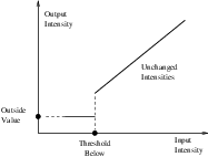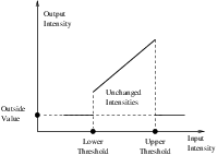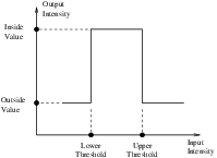
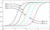
Figure 2.1: Transfer function of the BinaryThresholdImageFilter.
This chapter introduces the most commonly used filters found in the toolkit. Most of these filters are intended to process images. They will accept one or more images as input and will produce one or more images as output. ITK is based on a data pipeline architecture in which the output of one filter is passed as input to another filter. (See the Data Processing Pipeline section in Book 1 for more information.)
The thresholding operation is used to change or identify pixel values based on specifying one or more values (called the threshold value). The following sections describe how to perform thresholding operations using ITK.
The source code for this section can be found in the file
BinaryThresholdImageFilter.cxx.
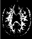
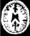
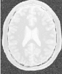
This example illustrates the use of the binary threshold image filter. This filter is used to transform an image into a binary image by changing the pixel values according to the rule illustrated in Figure 2.1. The user defines two thresholds—Upper and Lower—and two intensity values—Inside and Outside. For each pixel in the input image, the value of the pixel is compared with the lower and upper thresholds. If the pixel value is inside the range defined by [Lower,Upper] the output pixel is assigned the InsideValue. Otherwise the output pixels are assigned to the OutsideValue. Thresholding is commonly applied as the last operation of a segmentation pipeline.
The first step required to use the itk::BinaryThresholdImageFilter is to include its header file.
The next step is to decide which pixel types to use for the input and output images.
The input and output image types are now defined using their respective pixel types and dimensions.
The filter type can be instantiated using the input and output image types defined above.
An itk::ImageFileReader class is also instantiated in order to read image data from a file. (See Section 1 on page 3 for more information about reading and writing data.)
An itk::ImageFileWriter is instantiated in order to write the output image to a file.
Both the filter and the reader are created by invoking their New() methods and assigning the result to itk::SmartPointers.
The image obtained with the reader is passed as input to the BinaryThresholdImageFilter.
The method SetOutsideValue() defines the intensity value to be assigned to those pixels whose intensities are outside the range defined by the lower and upper thresholds. The method SetInsideValue() defines the intensity value to be assigned to pixels with intensities falling inside the threshold range.
The methods SetLowerThreshold() and SetUpperThreshold() define the range of the input image intensities that will be transformed into the InsideValue. Note that the lower and upper thresholds are values of the type of the input image pixels, while the inside and outside values are of the type of the output image pixels.
The execution of the filter is triggered by invoking the Update() method. If the filter’s output has been passed as input to subsequent filters, the Update() call on any downstream filters in the pipeline will indirectly trigger the update of this filter.


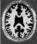
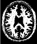
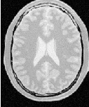
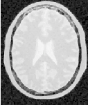
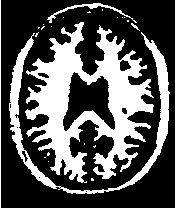
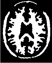
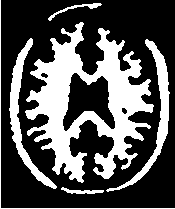
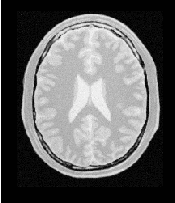
Figure 2.2 illustrates the effect of this filter on a MRI proton density image of the brain. This figure shows the limitations of the filter for performing segmentation by itself. These limitations are particularly noticeable in noisy images and in images lacking spatial uniformity as is the case with MRI due to field bias.
The following classes provide similar functionality:
The source code for this section can be found in the file
ThresholdImageFilter.cxx.
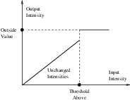
This example illustrates the use of the itk::ThresholdImageFilter. This filter can be used to transform the intensity levels of an image in three different ways.
The following methods choose among the three operating modes of the filter.
The first step required to use this filter is to include its header file.
Then we must decide what pixel type to use for the image. This filter is templated over a single image type because the algorithm only modifies pixel values outside the specified range, passing the rest through unchanged.
The image is defined using the pixel type and the dimension.
The filter can be instantiated using the image type defined above.
An itk::ImageFileReader class is also instantiated in order to read image data from a file.
An itk::ImageFileWriter is instantiated in order to write the output image to a file.
Both the filter and the reader are created by invoking their New() methods and assigning the result to SmartPointers.
The image obtained with the reader is passed as input to the itk::ThresholdImageFilter.
The method SetOutsideValue() defines the intensity value to be assigned to those pixels whose intensities are outside the range defined by the lower and upper thresholds.
The method ThresholdBelow() defines the intensity value below which pixels of the input image will be changed to the OutsideValue.
The filter is executed by invoking the Update() method. If the filter is part of a larger image processing pipeline, calling Update() on a downstream filter will also trigger update of this filter.
The output of this example is shown in Figure 2.3. The second operating mode of the filter is now enabled by calling the method ThresholdAbove().
Updating the filter with this new setting produces the output shown in Figure 2.4. The third operating mode of the filter is enabled by calling ThresholdOutside().
The output of this third, “band-pass” thresholding mode is shown in Figure 2.5.
The examples in this section also illustrate the limitations of the thresholding filter for performing segmentation by itself. These limitations are particularly noticeable in noisy images and in images lacking spatial uniformity, as is the case with MRI due to field bias.
The following classes provide similar functionality:
The source code for this section can be found in the file
CannyEdgeDetectionImageFilter.cxx.
This example introduces the use of the itk::CannyEdgeDetectionImageFilter. Canny edge detection is widely used for edge detection since it is the optimal solution satisfying the constraints of good sensitivity, localization and noise robustness. To achieve this end, Canny edge detection is implemented internally as a multi-stage algorithm, which involves Gaussian smoothing to remove noise, calculation of gradient magnitudes to localize edge features, non-maximum suppression to remove suprious features, and finally thresholding to yield a binary image. Though the specifics of this internal pipeline are largely abstracted from the user of the class, it is nonetheless beneficial to have a general understanding of these components so that parameters can be appropriately adjusted.
The first step required for using this filter is to include its header file.
In this example, images are read and written with unsigned char pixel type. However, Canny edge detection requires floating point pixel types in order to avoid numerical errors. For this reason, a separate internal image type with pixel type double is defined for edge detection.
The CharImageType image is cast to and from RealImageType using itk::CastImageFilter and RescaleIntensityImageFilter, respectively; both the input and output of CannyEdgeDetectionImageFilter are RealImageType.
In this example, three parameters of the Canny edge detection filter may be set via the SetVariance(), SetUpperThreshold(), and SetLowerThreshold() methods. Based on the previous discussion of the steps in the internal pipeline, we understand that variance adjusts the amount of Gaussian smoothing and upperThreshold and lowerThreshold control which edges are selected in the final step.
Finally, Update() is called on writer to trigger excecution of the pipeline. As usual, the call is wrapped in a try/catch block.
The filters discussed in this section perform pixel-wise intensity mappings. Casting is used to convert one pixel type to another, while intensity mappings also take into account the different intensity ranges of the pixel types.
The source code for this section can be found in the file
CastingImageFilters.cxx.
Due to the use of Generic Programming in the toolkit, most types are resolved at compile-time. Few decisions regarding type conversion are left to run-time. It is up to the user to anticipate the pixel type-conversions required in the data pipeline. In medical imaging applications it is usually not desirable to use a general pixel type since this may result in the loss of valuable information.
This section introduces the mechanisms for explicit casting of images that flow through the pipeline. The following four filters are treated in this section: itk::CastImageFilter, itk::RescaleIntensityImageFilter, itk::ShiftScaleImageFilter and itk::NormalizeImageFilter. These filters are not directly related to each other except that they all modify pixel values. They are presented together here for the purpose of comparing their individual features.
The CastImageFilter is a very simple filter that acts pixel-wise on an input image, casting every pixel to the type of the output image. Note that this filter does not perform any arithmetic operation on the intensities. Applying CastImageFilter is equivalent to performing a C-Style cast on every pixel.
outputPixel = static_cast<OutputPixelType>( inputPixel )
The RescaleIntensityImageFilter linearly scales the pixel values in such a way that the minimum and maximum values of the input are mapped to minimum and maximum values provided by the user. This is a typical process for forcing the dynamic range of the image to fit within a particular scale and is common for image display. The linear transformation applied by this filter can be expressed as

.
The ShiftScaleImageFilter also applies a linear transformation to the intensities of the input image, but the transformation is specified by the user in the form of a multiplying factor and a value to be added. This can be expressed as

.
The parameters of the linear transformation applied by the NormalizeImageFilter are computed internally such that the statistical distribution of gray levels in the output image have zero mean and a variance of one. This intensity correction is particularly useful in registration applications as a preprocessing step to the evaluation of mutual information metrics. The linear transformation of NormalizeImageFilter is given as
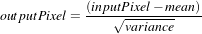
.
As usual, the first step required to use these filters is to include their header files.
Let’s define pixel types for the input and output images.
Then, the input and output image types are defined.
The filters are instantiated using the defined image types.
using CastFilterType = itk::CastImageFilter<
InputImageType, OutputImageType >;
using RescaleFilterType = itk::RescaleIntensityImageFilter<
InputImageType, OutputImageType >;
using ShiftScaleFilterType = itk::ShiftScaleImageFilter<
InputImageType, OutputImageType >;
using NormalizeFilterType = itk::NormalizeImageFilter<
InputImageType, OutputImageType >;
Object filters are created by invoking the New() method and assigning the result to itk::SmartPointers.
The output of a reader filter (whose creation is not shown here) is now connected as input to the various casting filters.
Next we proceed to setup the parameters required by each filter. The CastImageFilter and the NormalizeImageFilter do not require any parameters. The RescaleIntensityImageFilter, on the other hand, requires the user to provide the desired minimum and maximum pixel values of the output image. This is done by using the SetOutputMinimum() and SetOutputMaximum() methods as illustrated below.
The ShiftScaleImageFilter requires a multiplication factor (scale) and a post-scaling additive value (shift). The methods SetScale() and SetShift() are used, respectively, to set these values.
Finally, the filters are executed by invoking the Update() method.
The following filter can be seen as a variant of the casting filters. Its main difference is the use of a smooth and continuous transition function of non-linear form.
The source code for this section can be found in the file
SigmoidImageFilter.cxx.
The itk::SigmoidImageFilter is commonly used as an intensity transform. It maps a specific range of intensity values into a new intensity range by making a very smooth and continuous transition in the borders of the range. Sigmoids are widely used as a mechanism for focusing attention on a particular set of values and progressively attenuating the values outside that range. In order to extend the flexibility of the Sigmoid filter, its implementation in ITK includes four parameters that can be tuned to select its input and output intensity ranges. The following equation represents the Sigmoid intensity transformation, applied pixel-wise.
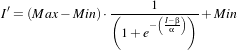 | (2.1) |
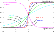
In the equation above, I is the intensity of the input pixel, I′ the intensity of the output pixel, Min,Max are the minimum and maximum values of the output image, α defines the width of the input intensity range, and β defines the intensity around which the range is centered. Figure 2.6 illustrates the significance of each parameter.
This filter will work on images of any dimension and will take advantage of multiple processors when available.
The header file corresponding to this filter should be included first.
Then pixel and image types for the filter input and output must be defined.
Using the image types, we instantiate the filter type and create the filter object.
The minimum and maximum values desired in the output are defined using the methods SetOutputMinimum() and SetOutputMaximum().
The coefficients α and β are set with the methods SetAlpha() and SetBeta(). Note that α is proportional to the width of the input intensity window. As rule of thumb, we may say that the window is the interval [-3α,3α]. The boundaries of the intensity window are not sharp. The α curve approaches its extrema smoothly, as shown in Figure 2.6. You may want to think about this in the same terms as when taking a range in a population of measures by defining an interval of [-3σ,+3σ] around the population mean.
The input to the SigmoidImageFilter can be taken from any other filter, such as an image file reader, for example. The output can be passed down the pipeline to other filters, like an image file writer. An Update() call on any downstream filter will trigger the execution of the Sigmoid filter.
Figure 2.7 illustrates the effect of this filter on a slice of MRI brain image using the following parameters.
As can be seen from the figure, the intensities of the white matter were expanded in their dynamic range, while intensity values lower than β-3α and higher than β+3α became progressively mapped to the minimum and maximum output values. This is the way in which a Sigmoid can be used for performing smooth intensity windowing.
Note that both α and β can be positive and negative. A negative α will have the effect of negating the image. This is illustrated on the left side of Figure 2.6. An application of the Sigmoid filter as preprocessing for segmentation is presented in Section 4.3.1.
Sigmoid curves are common in the natural world. They represent the plot of sensitivity to a stimulus. They are also the integral curve of the Gaussian and, therefore, appear naturally as the response to signals whose distribution is Gaussian.
Computation of gradients is a fairly common operation in image processing. The term “gradient” may refer in some contexts to the gradient vectors and in others to the magnitude of the gradient vectors. ITK filters attempt to reduce this ambiguity by including the magnitude term when appropriate. ITK provides filters for computing both the image of gradient vectors and the image of magnitudes.
The source code for this section can be found in the file
GradientMagnitudeImageFilter.cxx.
The magnitude of the image gradient is extensively used in image analysis, mainly to help in the determination of object contours and the separation of homogeneous regions. The itk::GradientMagnitudeImageFilter computes the magnitude of the image gradient at each pixel location using a simple finite differences approach. For example, in the case of 2D the computation is equivalent to convolving the image with masks of type
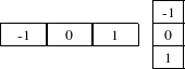
then adding the sum of their squares and computing the square root of the sum.
This filter will work on images of any dimension thanks to the internal use of itk::NeighborhoodIterator and itk::NeighborhoodOperator.
The first step required to use this filter is to include its header file.
Types should be chosen for the pixels of the input and output images.
The input and output image types can be defined using the pixel types.
The type of the gradient magnitude filter is defined by the input image and the output image types.
A filter object is created by invoking the New() method and assigning the result to a itk::SmartPointer.
The input image can be obtained from the output of another filter. Here, the source is an image reader.
Finally, the filter is executed by invoking the Update() method.
If the output of this filter has been connected to other filters in a pipeline, updating any of the downstream filters will also trigger an update of this filter. For example, the gradient magnitude filter may be connected to an image writer.

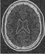
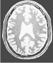
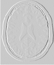
Figure 2.8 illustrates the effect of the gradient magnitude filter on a MRI proton density image of the brain. The figure shows the sensitivity of this filter to noisy data.
Attention should be paid to the image type chosen to represent the output image since the dynamic range of the gradient magnitude image is usually smaller than the dynamic range of the input image. As always, there are exceptions to this rule, for example, synthetic images that contain high contrast objects.
This filter does not apply any smoothing to the image before computing the gradients. The results can therefore be very sensitive to noise and may not be the best choice for scale-space analysis.
The source code for this section can be found in the file
GradientMagnitudeRecursiveGaussianImageFilter.cxx.
Differentiation is an ill-defined operation over digital data. In practice it is convenient to define a scale in which the differentiation should be performed. This is usually done by preprocessing the data with a smoothing filter. It has been shown that a Gaussian kernel is the most convenient choice for performing such smoothing. By choosing a particular value for the standard deviation (σ) of the Gaussian, an associated scale is selected that ignores high frequency content, commonly considered image noise.
The itk::GradientMagnitudeRecursiveGaussianImageFilter computes the magnitude of the image gradient at each pixel location. The computational process is equivalent to first smoothing the image by convolving it with a Gaussian kernel and then applying a differential operator. The user selects the value of σ.
Internally this is done by applying an IIR 1 filter that approximates a convolution with the derivative of the Gaussian kernel. Traditional convolution will produce a more accurate result, but the IIR approach is much faster, especially using large σs [15, 16].
GradientMagnitudeRecursiveGaussianImageFilter will work on images of any dimension by taking advantage of the natural separability of the Gaussian kernel and its derivatives.
The first step required to use this filter is to include its header file.
Types should be instantiated based on the pixels of the input and output images.
With them, the input and output image types can be instantiated.
The filter type is now instantiated using both the input image and the output image types.
A filter object is created by invoking the New() method and assigning the result to a itk::SmartPointer.
The input image can be obtained from the output of another filter. Here, an image reader is used as source.
The standard deviation of the Gaussian smoothing kernel is now set.
Finally the filter is executed by invoking the Update() method.
If connected to other filters in a pipeline, this filter will automatically update when any downstream filters are updated. For example, we may connect this gradient magnitude filter to an image file writer and then update the writer.
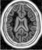
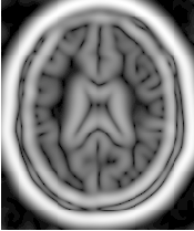
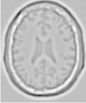
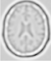
Figure 2.9 illustrates the effect of this filter on a MRI proton density image of the brain using σ values of 3 (left) and 5 (right). The figure shows how the sensitivity to noise can be regulated by selecting an appropriate σ. This type of scale-tunable filter is suitable for performing scale-space analysis.
Attention should be paid to the image type chosen to represent the output image since the dynamic range of the gradient magnitude image is usually smaller than the dynamic range of the input image.
The source code for this section can be found in the file
DerivativeImageFilter.cxx.
The itk::DerivativeImageFilter is used for computing the partial derivative of an image, the derivative of an image along a particular axial direction.
The header file corresponding to this filter should be included first.
Next, the pixel types for the input and output images must be defined and, with them, the image types can be instantiated. Note that it is important to select a signed type for the image, since the values of the derivatives will be positive as well as negative.
Using the image types, it is now possible to define the filter type and create the filter object.
The order of the derivative is selected with the SetOrder() method. The direction along which the derivative will be computed is selected with the SetDirection() method.
The input to the filter can be taken from any other filter, for example a reader. The output can be passed down the pipeline to other filters, for example, a writer. An Update() call on any downstream filter will trigger the execution of the derivative filter.
Figure 2.10 illustrates the effect of the DerivativeImageFilter on a slice of MRI brain image. The derivative is taken along the x direction. The sensitivity to noise in the image is evident from this result.
The source code for this section can be found in the file
SecondDerivativeRecursiveGaussianImageFilter.cxx.
This example illustrates how to compute second derivatives of a 3D image using the itk::RecursiveGaussianImageFilter.
It’s good to be able to compute the raw derivative without any smoothing, but this can be problematic in a medical imaging scenario, when images will often have a certain amount of noise. It’s almost always more desirable to include a smoothing step first, where an image is convolved with a Gaussian kernel in whichever directions the user desires a derivative. The nature of the Gaussian kernel makes it easy to combine these two steps into one, using an infinite impulse response (IIR) filter. In this example, all the second derivatives are computed independently in the same way, as if they were intended to be used for building the Hessian matrix of the image (a square matrix of second-order derivatives of an image, which is useful in many image processing techniques).
First, we will include the relevant header files: the itkRecursiveGaussianImageFilter, the image reader, writer, and duplicator.
Next, we declare our pixel type and output pixel type to be floats, and our image dimension to be 3.
Using these definitions, define the image types, reader and writer types, and duplicator types, which are templated over the pixel types and dimension. Then, instantiate the reader, writer, and duplicator with the New() method.
using ImageType = itk::Image< PixelType, Dimension >;
using OutputImageType = itk::Image< OutputPixelType, Dimension >;
using ReaderType = itk::ImageFileReader< ImageType >;
using WriterType = itk::ImageFileWriter< OutputImageType >;
using DuplicatorType = itk::ImageDuplicator< OutputImageType >;
using FilterType = itk::RecursiveGaussianImageFilter<
ImageType,
ImageType >;
ReaderType::Pointer reader = ReaderType::New();
WriterType::Pointer writer = WriterType::New();
DuplicatorType::Pointer duplicator = DuplicatorType::New();
Here we create three new filters. For each derivative we take, we will want to smooth in that direction first. So after the filters are created, each is given a dimension, and set to (in this example) the same sigma. Note that here, σ represents the standard deviation, whereas the itk::DiscreteGaussianImageFilter exposes the SetVariance method.
FilterType::Pointer ga = FilterType::New();
FilterType::Pointer gb = FilterType::New();
FilterType::Pointer gc = FilterType::New();
ga->SetDirection( 0 );
gb->SetDirection( 1 );
gc->SetDirection( 2 );
if( argc > 3 )
{
const float sigma = std::stod( argv[3] );
ga->SetSigma( sigma );
gb->SetSigma( sigma );
gc->SetSigma( sigma );
}
First we will compute the second derivative of the z-direction. In order to do this, we smooth in the x- and y- directions, and finally smooth and compute the derivative in the z-direction. Taking the zero-order derivative is equivalent to simply smoothing in that direction. This result is commonly notated Izz.
ga->SetZeroOrder();
gb->SetZeroOrder();
gc->SetSecondOrder();
ImageType::Pointer inputImage = reader->GetOutput();
ga->SetInput( inputImage );
gb->SetInput( ga->GetOutput() );
gc->SetInput( gb->GetOutput() );
duplicator->SetInputImage( gc->GetOutput() );
gc->Update();
duplicator->Update();
ImageType::Pointer Izz = duplicator->GetOutput();
Recall that gc is the filter responsible for taking the second derivative. We can now take advantage of the pipeline architecture and, without much hassle, switch the direction of gc and gb, so that gc now takes the derivatives in the y-direction. Now we only need to call Update() on gc to re-run the entire pipeline from ga to gc, obtaining the second-order derivative in the y-direction, which is commonly notated Iyy.
Now we switch the directions of gc with that of ga in order to take the derivatives in the x-direction. This will give us Ixx.
Now we can reset the directions to their original values, and compute first derivatives in different directions. Since we set both gb and gc to compute first derivatives, and ga to zero-order (which is only smoothing) we will obtain Iyz.
Here is how you may easily obtain Ixz.
For the sake of completeness, here is how you may compute Ixz and Ixy.
writer->SetInput( Ixz );
outputFileName = outputPrefix + "-Ixz.mhd";
writer->SetFileName( outputFileName.c_str() );
writer->Update();
ga->SetDirection( 2 );
gb->SetDirection( 0 );
gc->SetDirection( 1 );
ga->SetZeroOrder();
gb->SetFirstOrder();
gc->SetFirstOrder();
gc->Update();
duplicator->Update();
ImageType::Pointer Ixy = duplicator->GetOutput();
writer->SetInput( Ixy );
outputFileName = outputPrefix + "-Ixy.mhd";
writer->SetFileName( outputFileName.c_str() );
writer->Update();
The source code for this section can be found in the file
LaplacianRecursiveGaussianImageFilter1.cxx.
This example illustrates how to use the itk::RecursiveGaussianImageFilter for computing the Laplacian of a 2D image.
The first step required to use this filter is to include its header file.
Types should be selected on the desired input and output pixel types.
The input and output image types are instantiated using the pixel types.
The filter type is now instantiated using both the input image and the output image types.
This filter applies the approximation of the convolution along a single dimension. It is therefore necessary to concatenate several of these filters to produce smoothing in all directions. In this example, we create a pair of filters since we are processing a 2D image. The filters are created by invoking the New() method and assigning the result to a itk::SmartPointer.
We need two filters for computing the X component of the Laplacian and two other filters for computing the Y component.
Since each one of the newly created filters has the potential to perform filtering along any dimension, we have to restrict each one to a particular direction. This is done with the SetDirection() method.
The itk::RecursiveGaussianImageFilter can approximate the convolution with the Gaussian or with its first and second derivatives. We select one of these options by using the SetOrder() method. Note that the argument is an enum whose values can be ZeroOrder, FirstOrder and SecondOrder. For example, to compute the x partial derivative we should select FirstOrder for x and ZeroOrder for y. Here we want only to smooth in x and y, so we select ZeroOrder in both directions.
There are two typical ways of normalizing Gaussians depending on their application. For scale-space analysis it is desirable to use a normalization that will preserve the maximum value of the input. This normalization is represented by the following equation.
 | (2.2) |
In applications that use the Gaussian as a solution of the diffusion equation it is desirable to use a normalization that preserves the integral of the signal. This last approach can be seen as a conservation of mass principle. This is represented by the following equation.
 | (2.3) |
The itk::RecursiveGaussianImageFilter has a boolean flag that allows users to select between these two normalization options. Selection is done with the method SetNormalizeAcrossScale(). Enable this flag when analyzing an image across scale-space. In the current example, this setting has no impact because we are actually renormalizing the output to the dynamic range of the reader, so we simply disable the flag.
The input image can be obtained from the output of another filter. Here, an image reader is used as the source. The image is passed to the x filter and then to the y filter. The reason for keeping these two filters separate is that it is usual in scale-space applications to compute not only the smoothing but also combinations of derivatives at different orders and smoothing. Some factorization is possible when separate filters are used to generate the intermediate results. Here this capability is less interesting, though, since we only want to smooth the image in all directions.
It is now time to select the σ of the Gaussian used to smooth the data. Note that σ must be passed to both filters and that sigma is considered to be in millimeters. That is, at the moment of applying the smoothing process, the filter will take into account the spacing values defined in the image.
Finally the two components of the Laplacian should be added together. The itk::AddImageFilter is used for this purpose.
The filters are triggered by invoking Update() on the Add filter at the end of the pipeline.
The resulting image could be saved to a file using the itk::ImageFileWriter class.
The source code for this section can be found in the file
LaplacianRecursiveGaussianImageFilter2.cxx.
The previous example showed how to use the itk::RecursiveGaussianImageFilter for computing the equivalent of a Laplacian of an image after smoothing with a Gaussian. The elements used in this previous example have been packaged together in the itk::LaplacianRecursiveGaussianImageFilter in order to simplify its usage. This current example shows how to use this convenience filter for achieving the same results as the previous example.
The first step required to use this filter is to include its header file.
Types should be selected on the desired input and output pixel types.
The input and output image types are instantiated using the pixel types.
The filter type is now instantiated using both the input image and the output image types.
This filter packages all the components illustrated in the previous example. The filter is created by invoking the New() method and assigning the result to a itk::SmartPointer.
The option for normalizing across scale space can also be selected in this filter.
The input image can be obtained from the output of another filter. Here, an image reader is used as the source.
It is now time to select the σ of the Gaussian used to smooth the data. Note that σ must be passed to both filters and that sigma is considered to be in millimeters. That is, at the moment of applying the smoothing process, the filter will take into account the spacing values defined in the image.
Finally the pipeline is executed by invoking the Update() method.
The concept of locality is frequently encountered in image processing in the form of filters that compute every output pixel using information from a small region in the neighborhood of the input pixel. The classical form of these filters are the 3×3 filters in 2D images. Convolution masks based on these neighborhoods can perform diverse tasks ranging from noise reduction, to differential operations, to mathematical morphology.
The Insight Toolkit implements an elegant approach to neighborhood-based image filtering. The input image is processed using a special iterator called the itk::NeighborhoodIterator. This iterator is capable of moving over all the pixels in an image and, for each position, it can address the pixels in a local neighborhood. Operators are defined that apply an algorithmic operation in the neighborhood of the input pixel to produce a value for the output pixel. The following section describes some of the more commonly used filters that take advantage of this construction. (See the Iterators chapter in Book 1 for more information.)
The source code for this section can be found in the file
MeanImageFilter.cxx.
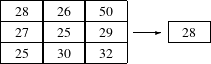
The itk::MeanImageFilter is commonly used for noise reduction. The filter computes the value of each output pixel by finding the statistical mean of the neighborhood of the corresponding input pixel. The following figure illustrates the local effect of the MeanImageFilter in a 2D case. The statistical mean of the neighborhood on the left is passed as the output value associated with the pixel at the center of the neighborhood.
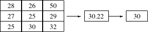
Note that this algorithm is sensitive to the presence of outliers in the neighborhood. This filter will work on images of any dimension thanks to the internal use of itk::SmartNeighborhoodIterator and itk::NeighborhoodOperator. The size of the neighborhood over which the mean is computed can be set by the user.
The header file corresponding to this filter should be included first.
Then the pixel types for input and output image must be defined and, with them, the image types can be instantiated.
Using the image types it is now possible to instantiate the filter type and create the filter object.
The size of the neighborhood is defined along every dimension by passing a SizeType object with the
corresponding values. The value on each dimension is used as the semi-size of a rectangular box. For
example, in 2D a size of  will result in a 3×5 neighborhood.
The input to the filter can be taken from any other filter, for example a reader. The output can be passed down the pipeline to other filters, for example, a writer. An update call on any downstream filter will trigger the execution of the mean filter.
Figure 2.12 illustrates the effect of this filter on a slice of MRI brain image using neighborhood radii of
 which corresponds to a 3×3 classical neighborhood. It can be seen from this picture that edges are
rapidly degraded by the diffusion of intensity values among neighbors.
which corresponds to a 3×3 classical neighborhood. It can be seen from this picture that edges are
rapidly degraded by the diffusion of intensity values among neighbors.
The source code for this section can be found in the file
MedianImageFilter.cxx.
The itk::MedianImageFilter is commonly used as a robust approach for noise reduction. This filter is particularly efficient against salt-and-pepper noise. In other words, it is robust to the presence of gray-level outliers. MedianImageFilter computes the value of each output pixel as the statistical median of the neighborhood of values around the corresponding input pixel. The following figure illustrates the local effect of this filter in a 2D case. The statistical median of the neighborhood on the left is passed as the output value associated with the pixel at the center of the neighborhood.
This filter will work on images of any dimension thanks to the internal use of itk::NeighborhoodIterator and itk::NeighborhoodOperator. The size of the neighborhood over which the median is computed can be set by the user.
The header file corresponding to this filter should be included first.
Then the pixel and image types of the input and output must be defined.
Using the image types, it is now possible to define the filter type and create the filter object.
The size of the neighborhood is defined along every dimension by passing a SizeType object with the
corresponding values. The value on each dimension is used as the semi-size of a rectangular box. For
example, in 2D a size of  will result in a 3×5 neighborhood.
The input to the filter can be taken from any other filter, for example a reader. The output can be passed down the pipeline to other filters, for example, a writer. An update call on any downstream filter will trigger the execution of the median filter.
Figure 2.13 illustrates the effect of the MedianImageFilter filter on a slice of MRI brain image using a
neighborhood radius of  , which corresponds to a 3×3 classical neighborhood. The filtered image
demonstrates the moderate tendency of the median filter to preserve edges.
, which corresponds to a 3×3 classical neighborhood. The filtered image
demonstrates the moderate tendency of the median filter to preserve edges.
Mathematical morphology has proved to be a powerful resource for image processing and analysis [55]. ITK implements mathematical morphology filters using NeighborhoodIterators and itk::NeighborhoodOperators. The toolkit contains two types of image morphology algorithms: filters that operate on binary images and filters that operate on grayscale images.
The source code for this section can be found in the file
MathematicalMorphologyBinaryFilters.cxx.
The following section illustrates the use of filters that perform basic mathematical morphology operations on binary images. The itk::BinaryErodeImageFilter and itk::BinaryDilateImageFilter are described here. The filter names clearly specify the type of image on which they operate. The header files required to construct a simple example of the use of the mathematical morphology filters are included below.
The following code defines the input and output pixel types and their associated image types.
Mathematical morphology operations are implemented by applying an operator over the neighborhood of each input pixel. The combination of the rule and the neighborhood is known as structuring element. Although some rules have become de facto standards for image processing, there is a good deal of freedom as to what kind of algorithmic rule should be applied to the neighborhood. The implementation in ITK follows the typical rule of minimum for erosion and maximum for dilation.
The structuring element is implemented as a NeighborhoodOperator. In particular, the default structuring element is the itk::BinaryBallStructuringElement class. This class is instantiated using the pixel type and dimension of the input image.
The structuring element type is then used along with the input and output image types for instantiating the type of the filters.
The filters can now be created by invoking the New() method and assigning the result to itk::SmartPointers.
The structuring element is not a reference counted class. Thus it is created as a C++ stack object instead of using New() and SmartPointers. The radius of the neighborhood associated with the structuring element is defined with the SetRadius() method and the CreateStructuringElement() method is invoked in order to initialize the operator. The resulting structuring element is passed to the mathematical morphology filter through the SetKernel() method, as illustrated below.
A binary image is provided as input to the filters. This image might be, for example, the output of a binary threshold image filter.
The values that correspond to “objects” in the binary image are specified with the methods SetErodeValue() and SetDilateValue(). The value passed to these methods will be considered the value over which the dilation and erosion rules will apply.
The filter is executed by invoking its Update() method, or by updating any downstream filter, such as an image writer.
Figure 2.14 illustrates the effect of the erosion and dilation filters on a binary image from a MRI brain slice. The figure shows how these operations can be used to remove spurious details from segmented images.
The source code for this section can be found in the file
MathematicalMorphologyGrayscaleFilters.cxx.
The following section illustrates the use of filters for performing basic mathematical morphology operations on grayscale images. The itk::GrayscaleErodeImageFilter and itk::GrayscaleDilateImageFilter are covered in this example. The filter names clearly specify the type of image on which they operate. The header files required for a simple example of the use of grayscale mathematical morphology filters are presented below.
The following code defines the input and output pixel types and their associated image types.
Mathematical morphology operations are based on the application of an operator over a neighborhood of each input pixel. The combination of the rule and the neighborhood is known as structuring element. Although some rules have become the de facto standard in image processing there is a good deal of freedom as to what kind of algorithmic rule should be applied on the neighborhood. The implementation in ITK follows the typical rule of minimum for erosion and maximum for dilation.
The structuring element is implemented as a itk::NeighborhoodOperator. In particular, the default structuring element is the itk::BinaryBallStructuringElement class. This class is instantiated using the pixel type and dimension of the input image.
The structuring element type is then used along with the input and output image types for instantiating the type of the filters.
The filters can now be created by invoking the New() method and assigning the result to SmartPointers.
The structuring element is not a reference counted class. Thus it is created as a C++ stack object instead of using New() and SmartPointers. The radius of the neighborhood associated with the structuring element is defined with the SetRadius() method and the CreateStructuringElement() method is invoked in order to initialize the operator. The resulting structuring element is passed to the mathematical morphology filter through the SetKernel() method, as illustrated below.
A grayscale image is provided as input to the filters. This image might be, for example, the output of a reader.
The filter is executed by invoking its Update() method, or by updating any downstream filter, such as an image writer.
Figure 2.15 illustrates the effect of the erosion and dilation filters on a binary image from a MRI brain slice. The figure shows how these operations can be used to remove spurious details from segmented images.
Voting filters are quite a generic family of filters. In fact, both the Dilate and Erode filters from Mathematical Morphology are very particular cases of the broader family of voting filters. In a voting filter, the outcome of a pixel is decided by counting the number of pixels in its neighborhood and applying a rule to the result of that counting. For example, the typical implementation of erosion in terms of a voting filter will be to label a foreground pixel as background if the number of background neighbors is greater than or equal to 1. In this context, you could imagine variations of erosion in which the count could be changed to require at least 3 foreground pixels in its neighborhood.
One case of a voting filter is the BinaryMedianImageFilter. This filter is equivalent to applying a Median filter over a binary image. Having a binary image as input makes it possible to optimize the execution of the filter since there is no real need for sorting the pixels according to their frequency in the neighborhood.
The source code for this section can be found in the file
BinaryMedianImageFilter.cxx.
The itk::BinaryMedianImageFilter is commonly used as a robust approach for noise reduction. BinaryMedianImageFilter computes the value of each output pixel as the statistical median of the neighborhood of values around the corresponding input pixel. When the input images are binary, the implementation can be optimized by simply counting the number of pixels ON/OFF around the current pixel.
This filter will work on images of any dimension thanks to the internal use of itk::NeighborhoodIterator and itk::NeighborhoodOperator. The size of the neighborhood over which the median is computed can be set by the user.
The header file corresponding to this filter should be included first.
Then the pixel and image types of the input and output must be defined.
Using the image types, it is now possible to define the filter type and create the filter object.
The size of the neighborhood is defined along every dimension by passing a SizeType object with the
corresponding values. The value on each dimension is used as the semi-size of a rectangular box. For
example, in 2D a size of  will result in a 3×5 neighborhood.
The input to the filter can be taken from any other filter, for example a reader. The output can be passed down the pipeline to other filters, for example, a writer. An update call on any downstream filter will trigger the execution of the median filter.
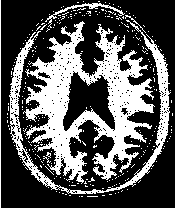
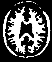
Figure 2.16 illustrates the effect of the BinaryMedianImageFilter filter on a slice of MRI brain image using
a neighborhood radius of  , which corresponds to a 5×5 classical neighborhood. The filtered image
demonstrates the capability of this filter for reducing noise both in the background and foreground of the
image, as well as smoothing the contours of the regions.
, which corresponds to a 5×5 classical neighborhood. The filtered image
demonstrates the capability of this filter for reducing noise both in the background and foreground of the
image, as well as smoothing the contours of the regions.
The typical effect of median filtration on a noisy digital image is a dramatic reduction in impulse noise spikes. The filter also tends to preserve brightness differences across signal steps, resulting in reduced blurring of regional boundaries. The filter also tends to preserve the positions of boundaries in an image.
Figure 2.17 below shows the effect of running the median filter with a 3x3 classical window size 1, 10 and 50 times. There is a tradeoff in noise reduction and the sharpness of the image when the window size is increased
.
Another variation of voting filters is the Hole Filling filter. This filter converts background pixels into foreground only when the number of foreground pixels is a majority of the neighbors. By selecting the size of the majority, this filter can be tuned to fill in holes of different sizes. To be more precise, the effect of the filter is actually related to the curvature of the edge in which the pixel is located.
The source code for this section can be found in the file
VotingBinaryHoleFillingImageFilter.cxx.
The itk::VotingBinaryHoleFillingImageFilter applies a voting operation in order to fill in cavities. This can be used for smoothing contours and for filling holes in binary images.
The header file corresponding to this filter should be included first.
Then the pixel and image types of the input and output must be defined.
Using the image types, it is now possible to define the filter type and create the filter object.
The size of the neighborhood is defined along every dimension by passing a SizeType object with the
corresponding values. The value on each dimension is used as the semi-size of a rectangular box. For
example, in 2D a size of  will result in a 3×5 neighborhood.
Since the filter is expecting a binary image as input, we must specify the levels that are going to be considered background and foreground. This is done with the SetForegroundValue() and SetBackgroundValue() methods.
We must also specify the majority threshold that is going to be used as the decision criterion for converting a background pixel into a foreground pixel. The rule of conversion is that a background pixel will be converted into a foreground pixel if the number of foreground neighbors surpass the number of background neighbors by the majority value. For example, in a 2D image, with neighborhood of radius 1, the neighborhood will have size 3×3. If we set the majority value to 2, then we are requiring that the number of foreground neighbors should be at least (3x3 -1 )/2 + majority. This is done with the SetMajorityThreshold() method.
The input to the filter can be taken from any other filter, for example a reader. The output can be passed down the pipeline to other filters, for example, a writer. An update call on any downstream filter will trigger the execution of the median filter.


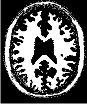
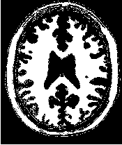
Figure 2.18 illustrates the effect of the VotingBinaryHoleFillingImageFilter filter on a thresholded slice of
MRI brain image using neighborhood radii of  ,
,  and
and  that correspond respectively to
neighborhoods of size 3×3, 5×5, 7×7. The filtered image demonstrates the capability of this filter for
reducing noise both in the background and foreground of the image, as well as smoothing the contours of
the regions.
that correspond respectively to
neighborhoods of size 3×3, 5×5, 7×7. The filtered image demonstrates the capability of this filter for
reducing noise both in the background and foreground of the image, as well as smoothing the contours of
the regions.
The Hole Filling filter can be used in an iterative way, by applying it repeatedly until no pixel changes. In this context, the filter can be seen as a binary variation of a Level Set filter.
The source code for this section can be found in the file
VotingBinaryIterativeHoleFillingImageFilter.cxx.
The itk::VotingBinaryIterativeHoleFillingImageFilter applies a voting operation in order to fill in cavities. This can be used for smoothing contours and for filling holes in binary images. This filter runs a itk::VotingBinaryHoleFillingImageFilter internally until no pixels change or the maximum number of iterations has been reached.
The header file corresponding to this filter should be included first.
Then the pixel and image types must be defined. Note that this filter requires the input and output images to be of the same type, therefore a single image type is required for the template instantiation.
Using the image types, it is now possible to define the filter type and create the filter object.
The size of the neighborhood is defined along every dimension by passing a SizeType object with the
corresponding values. The value on each dimension is used as the semi-size of a rectangular box. For
example, in 2D a size of  will result in a 3×5 neighborhood.
Since the filter is expecting a binary image as input, we must specify the levels that are going to be considered background and foreground. This is done with the SetForegroundValue() and SetBackgroundValue() methods.
We must also specify the majority threshold that is going to be used as the decision criterion for converting a background pixel into a foreground pixel. The rule of conversion is that a background pixel will be converted into a foreground pixel if the number of foreground neighbors surpass the number of background neighbors by the majority value. For example, in a 2D image, with neighborhood of radius 1, the neighborhood will have size 3×3. If we set the majority value to 2, then we are requiring that the number of foreground neighbors should be at least (3x3 -1 )/2 + majority. This is done with the SetMajorityThreshold() method.
Finally we specify the maximum number of iterations for which this filter should run. The number of iterations will determine the maximum size of holes and cavities that this filter will be able to fill. The more iterations you run, the larger the cavities that will be filled in.
The input to the filter can be taken from any other filter, for example a reader. The output can be passed down the pipeline to other filters, for example, a writer. An update call on any downstream filter will trigger the execution of the median filter.

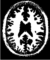
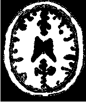
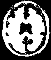
Figure 2.19 illustrates the effect of the VotingBinaryIterativeHoleFillingImageFilter filter on a thresholded
slice of MRI brain image using neighborhood radii of  ,
,  and
and  that correspond respectively to
neighborhoods of size 3×3, 5×5, 7×7. The filtered image demonstrates the capability of this filter for
reducing noise both in the background and foreground of the image, as well as smoothing the contours of
the regions.
that correspond respectively to
neighborhoods of size 3×3, 5×5, 7×7. The filtered image demonstrates the capability of this filter for
reducing noise both in the background and foreground of the image, as well as smoothing the contours of
the regions.
Real image data has a level of uncertainty which is manifested in the variability of measures assigned to pixels. This uncertainty is usually interpreted as noise and considered an undesirable component of the image data. This section describes several methods that can be applied to reduce noise on images.
Blurring is the traditional approach for removing noise from images. It is usually implemented in the form of a convolution with a kernel. The effect of blurring on the image spectrum is to attenuate high spatial frequencies. Different kernels attenuate frequencies in different ways. One of the most commonly used kernels is the Gaussian. Two implementations of Gaussian smoothing are available in the toolkit. The first one is based on a traditional convolution while the other is based on the application of IIR filters that approximate the convolution with a Gaussian [15, 16].
The source code for this section can be found in the file
DiscreteGaussianImageFilter.cxx.
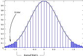
Figure 2.20: Discretized Gaussian.
The itk::DiscreteGaussianImageFilter computes the convolution of the input image with a Gaussian kernel. This is done in ND by taking advantage of the separability of the Gaussian kernel. A one-dimensional Gaussian function is discretized on a convolution kernel. The size of the kernel is extended until there are enough discrete points in the Gaussian to ensure that a user-provided maximum error is not exceeded. Since the size of the kernel is unknown a priori, it is necessary to impose a limit to its growth. The user can thus provide a value to be the maximum admissible size of the kernel. Discretization error is defined as the difference between the area under the discrete Gaussian curve (which has finite support) and the area under the continuous Gaussian.
Gaussian kernels in ITK are constructed according to the theory of Tony Lindeberg [34] so that smoothing and derivative operations commute before and after discretization. In other words, finite difference derivatives on an image I that has been smoothed by convolution with the Gaussian are equivalent to finite differences computed on I by convolving with a derivative of the Gaussian.
The first step required to use this filter is to include its header file. As with other examples, the includes here
are truncated to those specific for this example.
Types should be chosen for the pixels of the input and output images. Image types can be instantiated using the pixel type and dimension.
The discrete Gaussian filter type is instantiated using the input and output image types. A corresponding filter object is created.
The input image can be obtained from the output of another filter. Here, an image reader is used as its input.
The filter requires the user to provide a value for the variance associated with the Gaussian kernel. The method SetVariance() is used for this purpose. The discrete Gaussian is constructed as a convolution kernel. The maximum kernel size can be set by the user. Note that the combination of variance and kernel-size values may result in a truncated Gaussian kernel.
Finally, the filter is executed by invoking the Update() method.
If the output of this filter has been connected to other filters down the pipeline, updating any of the downstream filters will trigger the execution of this one. For example, a writer could be used after the filter.

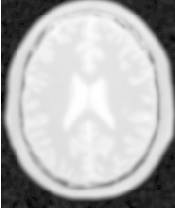
Figure 2.21 illustrates the effect of this filter on a MRI proton density image of the brain.
Note that large Gaussian variances will produce large convolution kernels and correspondingly longer computation times. Unless a high degree of accuracy is required, it may be more desirable to use the approximating itk::RecursiveGaussianImageFilter with large variances.
The source code for this section can be found in the file
BinomialBlurImageFilter.cxx.
The itk::BinomialBlurImageFilter computes a nearest neighbor average along each dimension. The process is repeated a number of times, as specified by the user. In principle, after a large number of iterations the result will approach the convolution with a Gaussian.
The first step required to use this filter is to include its header file.
Types should be chosen for the pixels of the input and output images. Image types can be instantiated using the pixel type and dimension.
The filter type is now instantiated using both the input image and the output image types. Then a filter object is created.
The input image can be obtained from the output of another filter. Here, an image reader is used as the source. The number of repetitions is set with the SetRepetitions() method. Computation time will increase linearly with the number of repetitions selected. Finally, the filter can be executed by calling the Update() method.


Figure 2.22 illustrates the effect of this filter on a MRI proton density image of the brain.
Note that the standard deviation σ of the equivalent Gaussian is fixed. In the spatial spectrum, the effect of every iteration of this filter is like a multiplication with a sinus cardinal function.
The source code for this section can be found in the file
SmoothingRecursiveGaussianImageFilter.cxx.
The classical method of smoothing an image by convolution with a Gaussian kernel has the drawback that it is slow when the standard deviation σ of the Gaussian is large. This is due to the larger size of the kernel, which results in a higher number of computations per pixel.
The itk::RecursiveGaussianImageFilter implements an approximation of convolution with the Gaussian and its derivatives by using IIR2 filters. In practice this filter requires a constant number of operations for approximating the convolution, regardless of the σ value [15, 16].
The first step required to use this filter is to include its header file.
Types should be selected on the desired input and output pixel types.
The input and output image types are instantiated using the pixel types.
The filter type is now instantiated using both the input image and the output image types.
This filter applies the approximation of the convolution along a single dimension. It is therefore necessary to concatenate several of these filters to produce smoothing in all directions. In this example, we create a pair of filters since we are processing a 2D image. The filters are created by invoking the New() method and assigning the result to a itk::SmartPointer.
Since each one of the newly created filters has the potential to perform filtering along any dimension, we have to restrict each one to a particular direction. This is done with the SetDirection() method.
The itk::RecursiveGaussianImageFilter can approximate the convolution with the Gaussian or with its first and second derivatives. We select one of these options by using the SetOrder() method. Note that the argument is an enum whose values can be ZeroOrder, FirstOrder and SecondOrder. For example, to compute the x partial derivative we should select FirstOrder for x and ZeroOrder for y. Here we want only to smooth in x and y, so we select ZeroOrder in both directions.
There are two typical ways of normalizing Gaussians depending on their application. For scale-space analysis it is desirable to use a normalization that will preserve the maximum value of the input. This normalization is represented by the following equation.
 | (2.4) |
In applications that use the Gaussian as a solution of the diffusion equation it is desirable to use a normalization that preserve the integral of the signal. This last approach can be seen as a conservation of mass principle. This is represented by the following equation.
 | (2.5) |
The itk::RecursiveGaussianImageFilter has a boolean flag that allows users to select between these two normalization options. Selection is done with the method SetNormalizeAcrossScale(). Enable this flag to analyzing an image across scale-space. In the current example, this setting has no impact because we are actually renormalizing the output to the dynamic range of the reader, so we simply disable the flag.
The input image can be obtained from the output of another filter. Here, an image reader is used as the source. The image is passed to the x filter and then to the y filter. The reason for keeping these two filters separate is that it is usual in scale-space applications to compute not only the smoothing but also combinations of derivatives at different orders and smoothing. Some factorization is possible when separate filters are used to generate the intermediate results. Here this capability is less interesting, though, since we only want to smooth the image in all directions.
It is now time to select the σ of the Gaussian used to smooth the data. Note that σ must be passed to both filters and that sigma is considered to be in millimeters. That is, at the moment of applying the smoothing process, the filter will take into account the spacing values defined in the image.
Finally the pipeline is executed by invoking the Update() method.
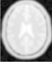
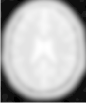
Figure 2.23 illustrates the effect of this filter on a MRI proton density image of the brain using σ values of 3 (left) and 5 (right). The figure shows how the attenuation of noise can be regulated by selecting the appropriate standard deviation. This type of scale-tunable filter is suitable for performing scale-space analysis.
The RecursiveGaussianFilters can also be applied on multi-component images. For instance, the above filter could have applied with RGBPixel as the pixel type. Each component is then independently filtered. However the RescaleIntensityImageFilter will not work on RGBPixels since it does not mathematically make sense to rescale the output of multi-component images.
In some cases it is desirable to compute smoothing in restricted regions of the image, or to do it using different parameters that are computed locally. The following sections describe options for applying local smoothing in images.
The source code for this section can be found in the file
GaussianBlurImageFunction.cxx.
The drawback of image denoising (smoothing) is that it tends to blur away the sharp boundaries in the image that help to distinguish between the larger-scale anatomical structures that one is trying to characterize (which also limits the size of the smoothing kernels in most applications). Even in cases where smoothing does not obliterate boundaries, it tends to distort the fine structure of the image and thereby changes subtle aspects of the anatomical shapes in question.
Perona and Malik [45] introduced an alternative to linear-filtering that they called anisotropic diffusion. Anisotropic diffusion is closely related to the earlier work of Grossberg [22], who used similar nonlinear diffusion processes to model human vision. The motivation for anisotropic diffusion (also called nonuniform or variable conductance diffusion) is that a Gaussian smoothed image is a single time slice of the solution to the heat equation, that has the original image as its initial conditions. Thus, the solution to
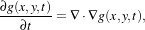 | (2.6) |
where g(x,y,0) = f(x,y) is the input image, is g(x,y,t) = G( )⊗f(x,y), where G(σ) is a Gaussian with
standard deviation σ.
)⊗f(x,y), where G(σ) is a Gaussian with
standard deviation σ.
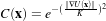
Anisotropic diffusion includes a variable conductance term that, in turn, depends on the differential structure of the image. Thus, the variable conductance can be formulated to limit the smoothing at “edges” in images, as measured by high gradient magnitude, for example.
 | (2.7) |
where, for notational convenience, we leave off the independent parameters of g and use the subscripts with respect to those parameters to indicate partial derivatives. The function c(|∇g|) is a fuzzy cutoff that reduces the conductance at areas of large |∇g|, and can be any one of a number of functions. The literature has shown
 | (2.8) |
to be quite effective. Notice that conductance term introduces a free parameter k, the conductance parameter, that controls the sensitivity of the process to edge contrast. Thus, anisotropic diffusion entails two free parameters: the conductance parameter, k, and the time parameter, t, that is analogous to σ, the effective width of the filter when using Gaussian kernels.
Equation 2.7 is a nonlinear partial differential equation that can be solved on a discrete grid using finite forward differences. Thus, the smoothed image is obtained only by an iterative process, not a convolution or non-stationary, linear filter. Typically, the number of iterations required for practical results are small, and large 2D images can be processed in several tens of seconds using carefully written code running on modern, general purpose, single-processor computers. The technique applies readily and effectively to 3D images, but requires more processing time.
In the early 1990’s several research groups [21, 67] demonstrated the effectiveness of anisotropic diffusion on medical images. In a series of papers on the subject [71, 69, 70, 67, 68, 65], Whitaker described a detailed analytical and empirical analysis, introduced a smoothing term in the conductance that made the process more robust, invented a numerical scheme that virtually eliminated directional artifacts in the original algorithm, and generalized anisotropic diffusion to vector-valued images, an image processing technique that can be used on vector-valued medical data (such as the color cryosection data of the Visible Human Project).
For a vector-valued input  : U
: U ℜm the process takes the form
 | (2.9) |
where 
 is a dissimilarity measure of
  , a generalization of the gradient magnitude to vector-valued
images, that can incorporate linear and nonlinear coordinate transformations on the range of
, a generalization of the gradient magnitude to vector-valued
images, that can incorporate linear and nonlinear coordinate transformations on the range of  . In this way,
the smoothing of the multiple images associated with vector-valued data is coupled through the
conductance term, that fuses the information in the different images. Thus vector-valued, nonlinear
diffusion can combine low-level image features (e.g. edges) across all “channels” of a vector-valued image
in order to preserve or enhance those features in all of image “channels”.
. In this way,
the smoothing of the multiple images associated with vector-valued data is coupled through the
conductance term, that fuses the information in the different images. Thus vector-valued, nonlinear
diffusion can combine low-level image features (e.g. edges) across all “channels” of a vector-valued image
in order to preserve or enhance those features in all of image “channels”.
Vector-valued anisotropic diffusion is useful for denoising data from devices that produce multiple values such as MRI or color photography. When performing nonlinear diffusion on a color image, the color channels are diffused separately, but linked through the conductance term. Vector-valued diffusion is also useful for processing registered data from different devices or for denoising higher-order geometric or statistical features from scalar-valued images [65, 72].
The output of anisotropic diffusion is an image or set of images that demonstrates reduced noise and texture but preserves, and can also enhance, edges. Such images are useful for a variety of processes including statistical classification, visualization, and geometric feature extraction. Previous work has shown [68] that anisotropic diffusion, over a wide range of conductance parameters, offers quantifiable advantages over linear filtering for edge detection in medical images.
Since the effectiveness of nonlinear diffusion was first demonstrated, numerous variations of this approach have surfaced in the literature [60]. These include alternatives for constructing dissimilarity measures [53], directional (i.e., tensor-valued) conductance terms [64, 3] and level set interpretations [66].
The source code for this section can be found in the file
GradientAnisotropicDiffusionImageFilter.cxx.
The itk::GradientAnisotropicDiffusionImageFilter implements an N-dimensional version of the classic Perona-Malik anisotropic diffusion equation for scalar-valued images [45].
The conductance term for this implementation is chosen as a function of the gradient magnitude of the image at each point, reducing the strength of diffusion at edge pixels.
 | (2.10) |
The numerical implementation of this equation is similar to that described in the Perona-Malik paper [45], but uses a more robust technique for gradient magnitude estimation and has been generalized to N-dimensions.
The first step required to use this filter is to include its header file.
Types should be selected based on the pixel types required for the input and output images. The image types are defined using the pixel type and the dimension.
The filter type is now instantiated using both the input image and the output image types. The filter object is created by the New() method.
The input image can be obtained from the output of another filter. Here, an image reader is used as source.
This filter requires three parameters: the number of iterations to be performed, the time step and the conductance parameter used in the computation of the level set evolution. These parameters are set using the methods SetNumberOfIterations(), SetTimeStep() and SetConductanceParameter() respectively. The filter can be executed by invoking Update().
Typical values for the time step are 0.25 in 2D images and 0.125 in 3D images. The number of iterations is typically set to 5; more iterations result in further smoothing and will increase the computing time linearly.


Figure 2.24 illustrates the effect of this filter on a MRI proton density image of the brain. In this example the filter was run with a time step of 0.25, and 5 iterations. The figure shows how homogeneous regions are smoothed and edges are preserved.
The following classes provide similar functionality:
The source code for this section can be found in the file
CurvatureAnisotropicDiffusionImageFilter.cxx.
The itk::CurvatureAnisotropicDiffusionImageFilter performs anisotropic diffusion on an image using a modified curvature diffusion equation (MCDE).
MCDE does not exhibit the edge enhancing properties of classic anisotropic diffusion, which can under certain conditions undergo a “negative” diffusion, which enhances the contrast of edges. Equations of the form of MCDE always undergo positive diffusion, with the conductance term only varying the strength of that diffusion.
Qualitatively, MCDE compares well with other non-linear diffusion techniques. It is less sensitive to contrast than classic Perona-Malik style diffusion, and preserves finer detailed structures in images. There is a potential speed trade-off for using this function in place of itkGradientNDAnisotropicDiffusionFunction. Each iteration of the solution takes roughly twice as long. Fewer iterations, however, may be required to reach an acceptable solution.
The MCDE equation is given as:
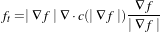 | (2.11) |
where the conductance modified curvature term is
 | (2.12) |
The first step required for using this filter is to include its header file.
Types should be selected based on the pixel types required for the input and output images. The image types are defined using the pixel type and the dimension.
The filter type is now instantiated using both the input image and the output image types. The filter object is created by the New() method.
The input image can be obtained from the output of another filter. Here, an image reader is used as source.
This filter requires three parameters: the number of iterations to be performed, the time step used in the computation of the level set evolution and the value of conductance. These parameters are set using the methods SetNumberOfIterations(), SetTimeStep() and SetConductance() respectively. The filter can be executed by invoking Update().
Typical values for the time step are 0.125 in 2D images and 0.0625 in 3D images. The number of iterations can be usually around 5, more iterations will result in further smoothing and will increase the computing time linearly. The conductance parameter is usually around 3.0.

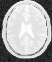
Figure 2.25 illustrates the effect of this filter on a MRI proton density image of the brain. In this example the filter was run with a time step of 0.125, 5 iterations and a conductance value of 3.0. The figure shows how homogeneous regions are smoothed and edges are preserved.
The following classes provide similar functionality:
The source code for this section can be found in the file
CurvatureFlowImageFilter.cxx.
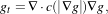
The itk::CurvatureFlowImageFilter performs edge-preserving smoothing in a similar fashion to the classical anisotropic diffusion. The filter uses a level set formulation where the iso-intensity contours in an image are viewed as level sets, where pixels of a particular intensity form one level set. The level set function is then evolved under the control of a diffusion equation where the speed is proportional to the curvature of the contour:
 | (2.13) |
where κ is the curvature.
Areas of high curvature will diffuse faster than areas of low curvature. Hence, small jagged noise artifacts will disappear quickly, while large scale interfaces will be slow to evolve, thereby preserving sharp boundaries between objects. However, it should be noted that although the evolution at the boundary is slow, some diffusion will still occur. Thus, continual application of this curvature flow scheme will eventually result in the removal of information as each contour shrinks to a point and disappears.
The first step required to use this filter is to include its header file.
Types should be selected based on the pixel types required for the input and output images.
With them, the input and output image types can be instantiated.
The CurvatureFlow filter type is now instantiated using both the input image and the output image types.
A filter object is created by invoking the New() method and assigning the result to a itk::SmartPointer.
The input image can be obtained from the output of another filter. Here, an image reader is used as source.
The CurvatureFlow filter requires two parameters: the number of iterations to be performed and the time step used in the computation of the level set evolution. These two parameters are set using the methods SetNumberOfIterations() and SetTimeStep() respectively. Then the filter can be executed by invoking Update().
Typical values for the time step are 0.125 in 2D images and 0.0625 in 3D images. The number of iterations can be usually around 10, more iterations will result in further smoothing and will increase the computing time linearly. Edge-preserving behavior is not guaranteed by this filter. Some degradation will occur on the edges and will increase as the number of iterations is increased.
If the output of this filter has been connected to other filters down the pipeline, updating any of the downstream filters will trigger the execution of this one. For example, a writer filter could be used after the curvature flow filter.

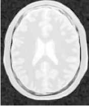
Figure 2.26 illustrates the effect of this filter on a MRI proton density image of the brain. In this example the filter was run with a time step of 0.25 and 10 iterations. The figure shows how homogeneous regions are smoothed and edges are preserved.
The following classes provide similar functionality:
The source code for this section can be found in the file
MinMaxCurvatureFlowImageFilter.cxx.
The MinMax curvature flow filter applies a variant of the curvature flow algorithm where diffusion is turned on or off depending of the scale of the noise that one wants to remove. The evolution speed is switched between min(κ,0) and max(κ,0) such that:
 | (2.14) |
where F is defined as
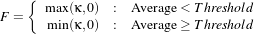 | (2.15) |
The Average is the average intensity computed over a neighborhood of a user-specified radius of the pixel. The choice of the radius governs the scale of the noise to be removed. The T hreshold is calculated as the average of pixel intensities along the direction perpendicular to the gradient at the extrema of the local neighborhood.
A speed of F = max(κ,0) will cause small dark regions in a predominantly light region to shrink. Conversely, a speed of F = min(κ,0), will cause light regions in a predominantly dark region to shrink. Comparison between the neighborhood average and the threshold is used to select the the right speed function to use. This switching prevents the unwanted diffusion of the simple curvature flow method.
Figure 2.27 shows the main elements involved in the computation. The set of square pixels represent the neighborhood over which the average intensity is being computed. The gray pixels are those lying close to the direction perpendicular to the gradient. The pixels which intersect the neighborhood bounds are used to compute the threshold value in the equation above. The integer radius of the neighborhood is selected by the user.
The first step required to use the itk::MinMaxCurvatureFlowImageFilter is to include its header file.
Types should be selected based on the pixel types required for the input and output images. The input and output image types are instantiated.
The itk::MinMaxCurvatureFlowImageFilter type is now instantiated using both the input image and the output image types. The filter is then created using the New() method.
The input image can be obtained from the output of another filter. Here, an image reader is used as source.
The itk::MinMaxCurvatureFlowImageFilter requires the two normal parameters of the CurvatureFlow image, the number of iterations to be performed and the time step used in the computation of the level set evolution. In addition, the radius of the neighborhood is also required. This last parameter is passed using the SetStencilRadius() method. Note that the radius is provided as an integer number since it is referring to a number of pixels from the center to the border of the neighborhood. Then the filter can be executed by invoking Update().
Typical values for the time step are 0.125 in 2D images and 0.0625 in 3D images. The number of iterations can be usually around 10, more iterations will result in further smoothing and will increase the computing time linearly. The radius of the stencil can be typically 1. The edge-preserving characteristic is not perfect on this filter. Some degradation will occur on the edges and will increase as the number of iterations is increased.
If the output of this filter has been connected to other filters down the pipeline, updating any of the downstream filters will trigger the execution of this one. For example, a writer filter can be used after the curvature flow filter.


Figure 2.28 illustrates the effect of this filter on a MRI proton density image of the brain. In this example the filter was run with a time step of 0.125, 10 iterations and a radius of 1. The figure shows how homogeneous regions are smoothed and edges are preserved. Notice also, that the result in the figure has sharper edges than the same example using simple curvature flow in Figure 2.26.
The following classes provide similar functionality:
The source code for this section can be found in the file
BilateralImageFilter.cxx.
The itk::BilateralImageFilter performs smoothing by using both domain and range neighborhoods. Pixels that are close to a pixel in the image domain and similar to a pixel in the image range are used to calculate the filtered value. Two Gaussian kernels (one in the image domain and one in the image range) are used to smooth the image. The result is an image that is smoothed in homogeneous regions yet has edges preserved. The result is similar to anisotropic diffusion but the implementation is non-iterative. Another benefit to bilateral filtering is that any distance metric can be used for kernel smoothing the image range. Bilateral filtering is capable of reducing the noise in an image by an order of magnitude while maintaining edges. The bilateral operator used here was described by Tomasi and Manduchi (Bilateral Filtering for Gray and Color Images. IEEE ICCV. 1998.)
The filtering operation can be described by the following equation
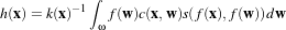 | (2.16) |
where x holds the coordinates of a ND point, f(x) is the input image and h(x) is the output image. The convolution kernels c() and s() are associated with the spatial and intensity domain respectively. The ND integral is computed over ω which is a neighborhood of the pixel located at x. The normalization factor k(x) is computed as
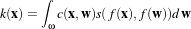 | (2.17) |
The default implementation of this filter uses Gaussian kernels for both c() and s(). The c kernel can be described as
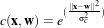 | (2.18) |
where σc is provided by the user and defines how close pixel neighbors should be in order to be considered for the computation of the output value. The s kernel is given by
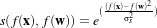 | (2.19) |
where σs is provided by the user and defines how close the neighbor’s intensity be in order to be considered for the computation of the output value.
The first step required to use this filter is to include its header file.
The image types are instantiated using pixel type and dimension.
The bilateral filter type is now instantiated using both the input image and the output image types and the filter object is created.
The input image can be obtained from the output of another filter. Here, an image reader is used as a source.
The Bilateral filter requires two parameters. First, we must specify the standard deviation σ to be used for the Gaussian kernel on image intensities. Second, the set of σs to be used along each dimension in the space domain. This second parameter is supplied as an array of float or double values. The array dimension matches the image dimension. This mechanism makes it possible to enforce more coherence along some directions. For example, more smoothing can be done along the X direction than along the Y direction.
In the following code example, the σ values are taken from the command line. Note the use of ImageType::ImageDimension to get access to the image dimension at compile time.
The filter parameters are set with the methods SetRangeSigma() and SetDomainSigma().
The output of the filter is connected here to a intensity rescaler filter and then to a writer. Invoking Update() on the writer triggers the execution of both filters.

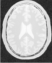
Figure 2.29 illustrates the effect of this filter on a MRI proton density image of the brain. In this example the filter was run with a range σ of 5.0 and a domain σ of 6.0. The figure shows how homogeneous regions are smoothed and edges are preserved.
The following classes provide similar functionality:
Anisotropic diffusion can also be applied to images whose pixels are vectors. In this case the diffusion is computed independently for each vector component. The following classes implement versions of anisotropic diffusion on vector images.
The source code for this section can be found in the file
VectorGradientAnisotropicDiffusionImageFilter.cxx.
The itk::VectorGradientAnisotropicDiffusionImageFilter implements an N-dimensional version of the classic Perona-Malik anisotropic diffusion equation for vector-valued images. Typically in vector-valued diffusion, vector components are diffused independently of one another using a conductance term that is linked across the components. The diffusion equation was illustrated in 2.7.3.
This filter is designed to process images of itk::Vector type. The code relies on various type alias and overloaded operators defined in itk::Vector. It is perfectly reasonable, however, to apply this filter to images of other, user-defined types as long as the appropriate type alias and operator overloads are in place. As a general rule, follow the example of itk::Vector in defining your data types.
The first step required to use this filter is to include its header file.
Types should be selected based on required pixel type for the input and output images. The image types are defined using the pixel type and the dimension.
The filter type is now instantiated using both the input image and the output image types. The filter object is created by the New() method.
The input image can be obtained from the output of another filter. Here, an image reader is used as source and its data is passed through a gradient filter in order to generate an image of vectors.
This filter requires two parameters: the number of iterations to be performed and the time step used in the computation of the level set evolution. These parameters are set using the methods SetNumberOfIterations() and SetTimeStep() respectively. The filter can be executed by invoking Update().
Typical values for the time step are 0.125 in 2D images and 0.0625 in 3D images. The number of iterations can be usually around 5, however more iterations will result in further smoothing and will linearly increase the computing time.

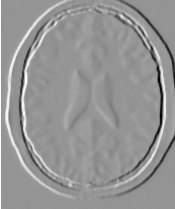
Figure 2.30 illustrates the effect of this filter on a MRI proton density image of the brain. The images show the X component of the gradient before (left) and after (right) the application of the filter. In this example the filter was run with a time step of 0.25, and 5 iterations.
The source code for this section can be found in the file
VectorCurvatureAnisotropicDiffusionImageFilter.cxx.
The itk::VectorCurvatureAnisotropicDiffusionImageFilter performs anisotropic diffusion on a vector image using a modified curvature diffusion equation (MCDE). The MCDE is the same described in 2.7.3.
Typically in vector-valued diffusion, vector components are diffused independently of one another using a conductance term that is linked across the components.
This filter is designed to process images of itk::Vector type. The code relies on various type alias and overloaded operators defined in itk::Vector. It is perfectly reasonable, however, to apply this filter to images of other, user-defined types as long as the appropriate type alias and operator overloads are in place. As a general rule, follow the example of the itk::Vector class in defining your data types.
The first step required to use this filter is to include its header file.
Types should be selected based on required pixel type for the input and output images. The image types are defined using the pixel type and the dimension.
The filter type is now instantiated using both the input image and the output image types. The filter object is created by the New() method.
The input image can be obtained from the output of another filter. Here, an image reader is used as source and its data is passed through a gradient filter in order to generate an image of vectors.
This filter requires two parameters: the number of iterations to be performed and the time step used in the computation of the level set evolution. These parameters are set using the methods SetNumberOfIterations() and SetTimeStep() respectively. The filter can be executed by invoking Update().
Typical values for the time step are 0.125 in 2D images and 0.0625 in 3D images. The number of iterations can be usually around 5, however more iterations will result in further smoothing and will increase the computing time linearly.
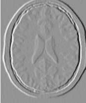
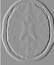
Figure 2.31 illustrates the effect of this filter on a MRI proton density image of the brain. The images show the X component of the gradient before (left) and after (right) the application of the filter. In this example the filter was run with a time step of 0.25, and 5 iterations.
The source code for this section can be found in the file
RGBGradientAnisotropicDiffusionImageFilter.cxx.
The vector anisotropic diffusion approach applies to color images equally well. As in the vector case, each RGB component is diffused independently. The following example illustrates the use of the Vector curvature anisotropic diffusion filter on an image with itk::RGBPixel type.
The first step required to use this filter is to include its header file.
Also the headers for Image and RGBPixel type are required.
It is desirable to perform the computation on the RGB image using float representation. However for input and output purposes unsigned char RGB components are commonly used. It is necessary to cast the type of color components along the pipeline before writing them to a file. The itk::CastImageFilter is used to achieve this goal.
The image type is defined using the pixel type and the dimension.
The filter type is now instantiated and a filter object is created by the New() method.
The input image can be obtained from the output of another filter. Here, an image reader is used as source.
This filter requires two parameters: the number of iterations to be performed and the time step used in the computation of the level set evolution. These parameters are set using the methods SetNumberOfIterations() and SetTimeStep() respectively. The filter can be executed by invoking Update().
The filter output is now cast to unsigned char RGB components by using the itk::CastImageFilter.
Finally, the writer type can be instantiated. One writer is created and connected to the output of the cast filter.
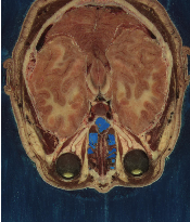
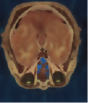
Figure 2.32 illustrates the effect of this filter on a RGB image from a cryogenic section of the Visible Woman data set. In this example the filter was run with a time step of 0.125, and 20 iterations. The input image has 570×670 pixels and the processing took 4 minutes on a Pentium 4 2GHz.
The source code for this section can be found in the file
RGBCurvatureAnisotropicDiffusionImageFilter.cxx.
The vector anisotropic diffusion approach can be applied equally well to color images. As in the vector case, each RGB component is diffused independently. The following example illustrates the use of the itk::VectorCurvatureAnisotropicDiffusionImageFilter on an image with itk::RGBPixel type.
The first step required to use this filter is to include its header file.
Also the headers for Image and RGBPixel type are required.
It is desirable to perform the computation on the RGB image using float representation. However for input and output purposes unsigned char RGB components are commonly used. It is necessary to cast the type of color components in the pipeline before writing them to a file. The itk::CastImageFilter is used to achieve this goal.
The image type is defined using the pixel type and the dimension.
The filter type is now instantiated and a filter object is created by the New() method.
The input image can be obtained from the output of another filter. Here, an image reader is used as a source.
This filter requires two parameters: the number of iterations to be performed and the time step used in the computation of the level set evolution. These parameters are set using the methods SetNumberOfIterations() and SetTimeStep() respectively. The filter can be executed by invoking Update().
The filter output is now cast to unsigned char RGB components by using the itk::CastImageFilter.
Finally, the writer type can be instantiated. One writer is created and connected to the output of the cast filter.


Figure 2.33 illustrates the effect of this filter on a RGB image from a cryogenic section of the Visible Woman data set. In this example the filter was run with a time step of 0.125, and 20 iterations. The input image has 570×670 pixels and the processing took 4 minutes on a Pentium 4 at 2GHz.


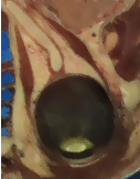
Figure 2.34 compares the effect of the gradient and curvature anisotropic diffusion filters on a small region of the same cryogenic slice used in Figure 2.33. The region used in this figure is only 127×162 pixels and took 14 seconds to compute on the same platform.
The source code for this section can be found in the file
DanielssonDistanceMapImageFilter.cxx.
This example illustrates the use of the itk::DanielssonDistanceMapImageFilter. This filter generates a distance map from the input image using the algorithm developed by Danielsson [13]. As secondary outputs, a Voronoi partition of the input elements is produced, as well as a vector image with the components of the distance vector to the closest point. The input to the map is assumed to be a set of points on the input image. The label of each group of pixels is assigned by the itk::ConnectedComponentImageFilter.
The first step required to use this filter is to include its header file.
Then we must decide what pixel types to use for the input and output images. Since the output will contain distances measured in pixels, the pixel type should be able to represent at least the width of the image, or said in N-dimensional terms, the maximum extension along all the dimensions. The input, output (distance map), and voronoi partition image types are now defined using their respective pixel type and dimension.
The filter type can be instantiated using the input and output image types defined above. A filter object is created with the New() method.
The input to the filter is taken from a reader and its output is passed to a itk::RescaleIntensityImageFilter and then to a writer. The scaler and writer are both templated over the image type, so we instantiate a separate pipeline for the voronoi partition map starting at the scaler.
The Voronoi map is obtained with the GetVoronoiMap() method. In the lines below we connect this output to the intensity rescaler.
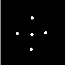
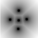
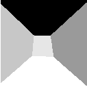
Figure 2.35 illustrates the effect of this filter on a binary image with a set of points. The input image is shown at the left, and the distance map at the center and the Voronoi partition at the right. This filter computes distance maps in N-dimensions and is therefore capable of producing N-dimensional Voronoi partitions.
The distance filter also produces an image of itk::Offset pixels representing the vectorial distance to the closest object in the scene. The type of this output image is defined by the VectorImageType trait of the filter type.
We can use this type for instantiating an itk::ImageFileWriter type and creating an object of this class in the following lines.
The output of the distance filter can be connected as input to the writer.
Execution of the writer is triggered by the invocation of the Update() method. Since this method can potentially throw exceptions it must be placed in a try/catch block.
Note that only the itk::MetaImageIO class supports reading and writing images of pixel type itk::Offset.
The source code for this section can be found in the file
SignedDanielssonDistanceMapImageFilter.cxx.
This example illustrates the use of the itk::SignedDanielssonDistanceMapImageFilter. This filter generates a distance map by running Danielsson distance map twice, once on the input image and once on the flipped image.
The first step required to use this filter is to include its header file.
Then we must decide what pixel types to use for the input and output images. Since the output will contain distances measured in pixels, the pixel type should be able to represent at least the width of the image, or said in N-dimensional terms, the maximum extension along all the dimensions. The input and output image types are now defined using their respective pixel type and dimension.
using InputPixelType = unsigned char;
using OutputPixelType = float;
using VoronoiPixelType = unsigned short;
constexpr unsigned int Dimension = 2;
using InputImageType = itk::Image< InputPixelType, Dimension >;
using OutputImageType = itk::Image< OutputPixelType, Dimension >;
using VoronoiImageType = itk::Image< VoronoiPixelType, Dimension >;
The only change with respect to the previous example is to replace the DanielssonDistanceMapImageFilter with the SignedDanielssonDistanceMapImageFilter.
The distances inside the circle are defined to be negative, while the distances outside the circle are positive. To change the convention, use the InsideIsPositive(bool) function.

Figure 2.36 illustrates the effect of this filter. The input image and the distance map are shown.
This one is the scariest and most dangerous filter in the entire toolkit. You should not use this filter unless you are entirely certain that you know what you are doing. In fact if you decide to use this filter, you should write your code, then go for a long walk, get more coffee and ask yourself if you really needed to use this filter. If the answer is yes, then you should discuss this issue with someone you trust and get his/her opinion in writing. In general, if you need to use this filter, it means that you have a poor image provider that is putting your career at risk along with the life of any potential patient whose images you may end up processing.
The source code for this section can be found in the file
FlipImageFilter.cxx.
The itk::FlipImageFilter is used for flipping the image content in any of the coordinate axes. This filter must be used with EXTREME caution. You probably don’t want to appear in the newspapers as responsible for a surgery mistake in which a doctor extirpates the left kidney when he should have extracted the right one3 . If that prospect doesn’t scare you, maybe it is time for you to reconsider your career in medical image processing. Flipping effects which seem innocuous at first view may still have dangerous consequences. For example, flipping the cranio-caudal axis of a CT scan forces an observer to flip the left-right axis in order to make sense of the image.
The header file corresponding to this filter should be included first.
Then the pixel types for input and output image must be defined and, with them, the image types can be instantiated.
Using the image types it is now possible to instantiate the filter type and create the filter object.
The axes to flip are specified in the form of an Array. In this case we take them from the command line arguments.
The input to the filter can be taken from any other filter, for example a reader. The output can be passed down the pipeline to other filters, for example, a writer. Invoking Update() on any downstream filter will trigger the execution of the FlipImage filter.
Figure 2.37 illustrates the effect of this filter on a slice of an MRI brain image using a flip array [0,1] which means that the Y axis was flipped while the X axis was conserved.
The source code for this section can be found in the file
ResampleImageFilter.cxx.
Resampling an image is a very important task in image analysis. It is especially important in the frame of image registration. The itk::ResampleImageFilter implements image resampling through the use of itk::Transforms. The inputs expected by this filter are an image, a transform and an interpolator. The space coordinates of the image are mapped through the transform in order to generate a new image. The extent and spacing of the resulting image are selected by the user. Resampling is performed in space coordinates, not pixel/grid coordinates. It is quite important to ensure that image spacing is properly set on the images involved. The interpolator is required since the mapping from one space to the other will often require evaluation of the intensity of the image at non-grid positions.
The header file corresponding to this filter should be included first.
The header files corresponding to the transform and interpolator must also be included.
The dimension and pixel types for input and output image must be defined and with them the image types can be instantiated.
Using the image and transform types it is now possible to instantiate the filter type and create the filter object.
The transform type is typically defined using the image dimension and the type used for representing space coordinates.
An instance of the transform object is instantiated and passed to the resample filter. By default, the parameters of the transform are set to represent the identity transform.
The interpolator type is defined using the full image type and the type used for representing space coordinates.
An instance of the interpolator object is instantiated and passed to the resample filter.
Given that some pixels of the output image may end up being mapped outside the extent of the input image it is necessary to decide what values to assign to them. This is done by invoking the SetDefaultPixelValue() method.
The sampling grid of the output space is specified with the spacing along each dimension and the origin.
The extent of the sampling grid on the output image is defined by a SizeType and is set using the SetSize() method.
The input to the filter can be taken from any other filter, for example a reader. The output can be passed down the pipeline to other filters, for example a writer. An update call on any downstream filter will trigger the execution of the resampling filter.
Figure 2.38 illustrates the effect of this filter on a slice of MRI brain image using an affine transform containing an identity transform. Note that any analysis of the behavior of this filter must be done on the space coordinate system in millimeters, not with respect to the sampling grid in pixels. The figure shows the resulting image in the lower left quarter of the extent. This may seem odd if analyzed in terms of the image grid but is quite clear when seen with respect to space coordinates. Figure 2.38 is particularly misleading because the images are rescaled to fit nicely on the text of this book. Figure 2.39 clarifies the situation. It shows the two same images placed on an equally-scaled coordinate system. It becomes clear here that an identity transform is being used to map the image data, and that simply, we have requested to resample additional empty space around the image. The input image is 181×217 pixels in size and we have requested an output of 300×300 pixels. In this case, the input and output images both have spacing of 1mm×1mm and origin of (0.0,0.0).
Let’s now set values on the transform. Note that the supplied transform represents the mapping of points from the output space to the input space. The following code sets up a translation.
The output image resulting from the translation can be seen in Figure 2.40. Again, it is better to interpret the result in a common coordinate system as illustrated in Figure 2.41.
Probably the most important thing to keep in mind when resampling images is that the transform is used to map points from the output image space into the input image space. In this case, Figure 2.41 shows that the translation is applied to every point of the output image and the resulting position is used to read the intensity from the input image. In this way, the gray level of the point P in the output image is taken from the point T (P) in the input image. Where T is the transformation. In the specific case of the Figure 2.41, the value of point (105,188) in the output image is taken from the point (75,138) of the input image because the transformation applied was a translation of (-30,-50).
It is sometimes useful to intentionally set the default output value to a distinct gray value in order to highlight the mapping of the image borders. For example, the following code sets the default external value of 100. The result is shown in the right side of Figure 2.42.
With this change we can better appreciate the effect of the previous translation transform on the image resampling. Figure 2.42 illustrates how the point (30,50) of the output image gets its gray value from the point (0,0) of the input image.
The source code for this section can be found in the file
ResampleImageFilter2.cxx.
During the computation of the resampled image all the pixels in the output region are visited. This visit is performed using ImageIterators which walk in the integer grid-space of the image. For each pixel, we need to convert grid position to space coordinates using the image spacing and origin.
For example, the pixel of index I = (20,50) in an image of origin O = (19.0,29.0) and pixel spacing S = (1.3,1.5) corresponds to the spatial position
![P[i]= I[i]× S[i]+ O[i]](ITKSoftwareGuide-Book2136x.png) | (2.20) |
which in this case leads to P = (20×1.3+19.0,50×1.5+29.0) and finally P = (45.0,104.0)
The space coordinates of P are mapped using the transform T supplied to the itk::ResampleImageFilter in order to map the point P to the input image space point Q = T (P).
The whole process is illustrated in Figure 2.43. In order to correctly interpret the process of the ResampleImageFilter you should be aware of the origin and spacing settings of both the input and output images.
In order to facilitate the interpretation of the transform we set the default pixel value to a value distinct from the image background.
Let’s set up a uniform spacing for the output image.
We will preserve the orientation of the input image by using the following call.
Additionally, we will specify a non-zero origin. Note that the values provided here will be those of the space coordinates for the pixel of index (0,0).
We set the transform to identity in order to better appreciate the effect of the origin selection.
The output resulting from these filter settings is analyzed in Figure 2.43.
In the figure, the output image point with index I = (0,0) has space coordinates P = (30,40). The identity transform maps this point to Q = (30,40) in the input image space. Because the input image in this case happens to have spacing (1.0,1.0) and origin (0.0,0.0), the physical point Q = (30,40) maps to the pixel with index I = (30,40).
The code for a different selection of origin and image size is illustrated below. The resulting output is presented in Figure 2.44.
The output image point with index I = (0,0) now has space coordinates P = (60,30). The identity transform maps this point to Q = (60,30) in the input image space. Because the input image in this case happens to have spacing (1.0,1.0) and origin (0.0,0.0), the physical point Q = (60,30) maps to the pixel with index I = (60,30).
Let’s now analyze the effect of a non-zero origin in the input image. Keeping the output image settings of the previous example, we modify only the origin values on the file header of the input image. The new origin assigned to the input image is O = (50,70). An identity transform is still used as input for the ResampleImageFilter. The result of executing the filter with these parameters is presented in Figure 2.45.
The pixel with index I = (56,120) on the output image has coordinates P = (116,150) in physical space. The identity transform maps P to the point Q = (116,150) on the input image space. The coordinates of Q are associated with the pixel of index I = (66,80) on the input image.
Now consider the effect of the output spacing on the process of image resampling. In order to simplify the analysis, let’s set the origin back to zero in both the input and output images.
We then specify a non-unit spacing for the output image.
Additionally, we reduce the output image extent, since the new pixels are now covering a larger area of 2.0mm ×3.0mm.
With these new parameters the physical extent of the output image is 160 millimeters by 150 millimeters.
Before attempting to analyze the effect of the resampling image filter it is important to make sure that the image viewer used to display the input and output images takes the spacing into account and appropriately scales the images on the screen. Please note that images in formats like PNG are not capable of representing origin and spacing. The toolkit assumes trivial default values for them. Figure 2.46 (center) illustrates the effect of using a naive viewer that does not take pixel spacing into account. A correct display is presented at the right in the same figure4 .

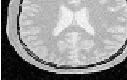
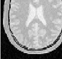
The filter output is analyzed in a common coordinate system with the input from Figure 2.47. In this figure, pixel I = (33,27) of the output image is located at coordinates P = (66.0,81.0) of the physical space. The identity transform maps this point to Q = (66.0,81.0) in the input image physical space. The point Q is then associated to the pixel of index I = (66,81) on the input image, because this image has zero origin and unit spacing.
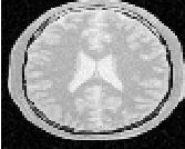
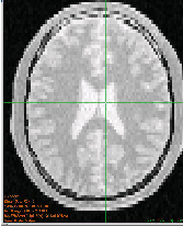
The input image spacing is also an important factor in the process of resampling an image. The following example illustrates the effect of non-unit pixel spacing on the input image. An input image similar to the those used in Figures 2.43 to 2.47 has been resampled to have pixel spacing of 2mm ×3mm. The input image is presented in Figure 2.48 as viewed with a naive image viewer (left) and with a correct image viewer (right).
The following code is used to transform this non-unit spacing input image into another non-unit spacing image located at a non-zero origin. The comparison between input and output in a common reference system is presented in figure 2.49.
Here we start by selecting the origin of the output image.
We then select the number of pixels along each dimension.
Finally, we set the output pixel spacing.
Figure 2.49 shows the analysis of the filter output under these conditions. First, notice that the origin of the output image corresponds to the settings O = (25.0,35.0) millimeters, spacing (4.0,4.5) millimeters and size (40,45) pixels. With these parameters the pixel of index I = (10,10) in the output image is associated with the spatial point of coordinates P = (10×4.0+25.0,10×4.5+35.0)) = (65.0,80.0). This point is mapped by the transform—identity in this particular case—to the point Q = (65.0,80.0) in the input image space. The point Q is then associated with the pixel of index I = ((65.0-0.0)∕2.0-(80.0-0.0)∕3.0) = (32.5,26.6). Note that the index does not fall on a grid position. For this reason the value to be assigned to the output pixel is computed by interpolating values on the input image around the non-integer index I = (32.5,26.6).
Note also that the discretization of the image is more visible on the output presented on the right side of Figure 2.49 due to the choice of a low resolution—just 40×45 pixels.
The source code for this section can be found in the file
ResampleImageFilter3.cxx.
Previous examples have described the basic principles behind the itk::ResampleImageFilter. Now it’s time to have some fun with it.
Figure 2.51 illustrates the general case of the resampling process. The origin and spacing of the output image has been selected to be different from those of the input image. The circles represent the center of pixels. They are inscribed in a rectangle representing the coverage of this pixel. The spacing specifies the distance between pixel centers along every dimension.
The transform applied is a rotation of 30 degrees. It is important to note here that the transform supplied to the itk::ResampleImageFilter is a clockwise rotation. This transform rotates the coordinate system of the output image 30 degrees clockwise. When the two images are relocated in a common coordinate system—as in Figure 2.51—the result is that the frame of the output image appears rotated 30 degrees clockwise. If the output image is seen with its coordinate system vertically aligned—as in Figure 2.50—the image content appears rotated 30 degrees counter-clockwise. Before continuing to read this section, you may want to meditate a bit on this fact while enjoying a cup of (Colombian) coffee.
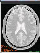
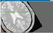
The following code implements the conditions illustrated in Figure 2.51 with two differences: the output spacing is 40 times smaller and there are 40 times more pixels in both dimensions. Without these changes, few details will be recognizable in the images. Note that the spacing and origin of the input image should be prepared in advance by using other means since this filter cannot alter the actual content of the input image in any way.
In order to facilitate the interpretation of the transform we set the default pixel value to value be distinct from the image background.
The spacing is selected here to be 40 times smaller than the one illustrated in Figure 2.51.
We will preserve the orientation of the input image by using the following call.
Let us now set up the origin of the output image. Note that the values provided here will be those of the space coordinates for the output image pixel of index (0,0).
The output image size is defined to be 40 times the one illustrated on the Figure 2.51.
Rotations are performed around the origin of physical coordinates—not the image origin nor the image center. Hence, the process of positioning the output image frame as it is shown in Figure 2.51 requires three steps. First, the image origin must be moved to the origin of the coordinate system. This is done by applying a translation equal to the negative values of the image origin.
In a second step, a rotation of 30 degrees is performed. In the itk::AffineTransform, angles are specified in radians. Also, a second boolean argument is used to specify if the current modification of the transform should be pre-composed or post-composed with the current transform content. In this case the argument is set to false to indicate that the rotation should be applied after the current transform content.
The third and final step implies translating the image origin back to its previous location. This is be done by applying a translation equal to the origin values.
Figure 2.50 presents the actual input and output images of this example as shown by a correct viewer which takes spacing into account. Note the clockwise versus counter-clockwise effect discussed previously between the representation in Figure 2.51 and Figure 2.50.
As a final exercise, let’s track the mapping of an individual pixel. Keep in mind that the transformation is initiated by walking through the pixels of the output image. This is the only way to ensure that the image will be generated without holes or redundant values. When you think about transformation it is always useful to analyze things from the output image towards the input image.
Let’s take the pixel with index I = (1,2) from the output image. The physical coordinates of this point in the output image reference system are P = (1×40.0+50.0,2×30.0+130.0) = (90.0,190.0) millimeters.
This point P is now mapped through the itk::AffineTransform into the input image space. The operation subtracts the origin, applies a 30 degrees rotation and adds the origin back. Let’s follow those steps. Subtracting the origin from P leads to P1 = (40.0,60.0), the rotation maps P1 to P2 = (40.0×cos(30.0)+60.0×sin(30.0),40.0×sin(30.0)-60.0×cos(30.0)) = (64.64,31.96). Finally this point is translated back by the amount of the image origin. This moves P2 to P3 = (114.64,161.96).
The point P3 is now in the coordinate system of the input image. The pixel of the input image associated with this physical position is computed using the origin and spacing of the input image. I = ((114.64-60.0)∕20.0,(161-70.0)∕30.0) which results in I = (2.7,3.0). Note that this is a non-grid position since the values are non-integers. This means that the gray value to be assigned to the output image pixel I = (1,2) must be computed by interpolation of the input image values.
In this particular code the interpolator used is simply a
itk::NearestNeighborInterpolateImageFunction which will assign the value of the
closest pixel. This ends up being the pixel of index I = (3,3) and can be seen from Figure
2.51.
The source code for this section can be found in the file
ResampleImageFilter4.cxx.
The following example illustrates how to rotate an image around its center. In this particular case an itk::AffineTransform is used to map the input space into the output space.
The header of the affine transform is included below.
The transform type is instantiated using the coordinate representation type and the space dimension. Then a transform object is constructed with the New() method and passed to a itk::SmartPointer.
The parameters of the output image are taken from the input image.
reader->Update();
const InputImageType ⋆ inputImage = reader->GetOutput();
const InputImageType::SpacingType & spacing = inputImage->GetSpacing();
const InputImageType::PointType & origin = inputImage->GetOrigin();
InputImageType::SizeType size =
inputImage->GetLargestPossibleRegion().GetSize();
filter->SetOutputOrigin( origin );
filter->SetOutputSpacing( spacing );
filter->SetOutputDirection( inputImage->GetDirection() );
filter->SetSize( size );
Rotations are performed around the origin of physical coordinates—not the image origin nor the image center. Hence, the process of positioning the output image frame as it is shown in Figure 2.52 requires three steps. First, the image origin must be moved to the origin of the coordinate system. This is done by applying a translation equal to the negative values of the image origin.
In a second step, the rotation is specified using the method Rotate2D().
The third and final step requires translating the image origin back to its previous location. This is be done by applying a translation equal to the origin values.
The output of the resampling filter is connected to a writer and the execution of the pipeline is triggered by a writer update.
The source code for this section can be found in the file
ResampleImageFilter5.cxx.
This example illustrates the use of the itk::Similarity2DTransform. A similarity transform involves rotation, translation and scaling. Since the parameterization of rotations is difficult to get in a generic ND case, a particular implementation is available for 2D.
The header file of the transform is included below.
The transform type is instantiated using the coordinate representation type as the single template parameter.
A transform object is constructed by calling New() and passing the result to a itk::SmartPointer.
The parameters of the output image are taken from the input image.
The Similarity2DTransform allows the user to select the center of rotation. This center is used for both rotation and scaling operations.
The rotation is specified with the method SetAngle().
The scale change is defined using the method SetScale().
A translation to be applied after the rotation and scaling can be specified with the method SetTranslation().
Note that the order in which rotation, scaling and translation are defined is irrelevant in this transform. This is not the case in the Affine transform which is very generic and allows different combinations for initialization. In the Similarity2DTransform class the rotation and scaling will always be applied before the translation.
Figure 2.53 shows the effect of this rotation, translation and scaling on a slice of a brain MRI. The scale applied for producing this figure was 1.2 and the rotation angle was 10∘.
The source code for this section can be found in the file
WarpImageFilter1.cxx.
This example illustrates how to use the WarpImageFilter and a deformation field for resampling an image. This is typically done as the last step of a deformable registration algorithm.
The deformation field is represented as an image of vector pixel types. The dimension of the vectors is the same as the dimension of the input image. Each vector in the deformation field represents the distance between a geometric point in the input space and a point in the output space such that:
 | (2.21) |
The field is read from a file, through a reader instantiated over the vector pixel types.
The itk::WarpImageFilter is templated over the input image type, output image type and the deformation field type.
Typically the mapped position does not correspond to an integer pixel position in the input image. Interpolation via an image function is used to compute values at non-integer positions. This is done via the SetInterpolator() method.
The output image spacing and origin may be set via SetOutputSpacing(), SetOutputOrigin(). This is taken from the deformation field.
The source code for this section can be found in the file
SubsampleVolume.cxx.
This example illustrates how to perform subsampling of a volume using ITK classes. In order to avoid aliasing artifacts, the volume must be processed by a low-pass filter before resampling. Here we use the itk::RecursiveGaussianImageFilter as a low-pass filter. The image is then resampled by using three different factors, one per dimension of the image.
The most important headers to include here are those corresponding to the resampling image filter, the transform, the interpolator and the smoothing filter.
We explicitly instantiate the pixel type and dimension of the input image, and the images that will be used internally for computing the resampling.
constexpr unsigned int Dimension = 3;
using InputPixelType = unsigned char;
using InternalPixelType = float;
using OutputPixelType = unsigned char;
using InputImageType = itk::Image< InputPixelType, Dimension >;
using InternalImageType = itk::Image< InternalPixelType, Dimension >;
using OutputImageType = itk::Image< OutputPixelType, Dimension >;
In this particular case we take the factors for resampling directly from the command line arguments.
A casting filter is instantiated in order to convert the pixel type of the input image into the pixel type desired for computing the resampling.
The smoothing filter of choice is the RecursiveGaussianImageFilter. We create three of them in order to have the freedom of performing smoothing with different sigma values along each dimension.
using GaussianFilterType = itk::RecursiveGaussianImageFilter<
InternalImageType,
InternalImageType >;
GaussianFilterType::Pointer smootherX = GaussianFilterType::New();
GaussianFilterType::Pointer smootherY = GaussianFilterType::New();
GaussianFilterType::Pointer smootherZ = GaussianFilterType::New();
The smoothing filters are connected in a cascade in the pipeline.
The sigma values to use in the smoothing filters are computed based on the pixel spacing of the input image and the factors provided as arguments.
const InputImageType::SpacingType& inputSpacing = inputImage->GetSpacing();
const double sigmaX = inputSpacing[0] ⋆ factorX;
const double sigmaY = inputSpacing[1] ⋆ factorY;
const double sigmaZ = inputSpacing[2] ⋆ factorZ;
smootherX->SetSigma( sigmaX );
smootherY->SetSigma( sigmaY );
smootherZ->SetSigma( sigmaZ );
We instruct each one of the smoothing filters to act along a particular direction of the image, and set them to use normalization across scale space in order to account for the reduction of intensity that accompanies the diffusion process associated with the Gaussian smoothing.
The type of the resampling filter is instantiated using the internal image type and the output image type.
Since the resampling is performed in the same physical extent of the input image, we select the IdentityTransform as the one to be used by the resampling filter.
The Linear interpolator is selected because it provides a good run-time performance. For applications that require better precision you may want to replace this interpolator with the itk::BSplineInterpolateImageFunction interpolator or with the itk::WindowedSincInterpolateImageFunction interpolator.
The spacing to be used in the grid of the resampled image is computed using the input image spacing and the factors provided in the command line arguments.
The origin and direction of the input image are both preserved and passed to the output image.
The number of pixels to use along each direction on the grid of the resampled image is computed using the number of pixels in the input image and the sampling factors.
InputImageType::SizeType inputSize =
inputImage->GetLargestPossibleRegion().GetSize();
using SizeValueType = InputImageType::SizeType::SizeValueType;
InputImageType::SizeType size;
size[0] = static_cast< SizeValueType >( inputSize[0] / factorX );
size[1] = static_cast< SizeValueType >( inputSize[1] / factorY );
size[2] = static_cast< SizeValueType >( inputSize[2] / factorZ );
resampler->SetSize( size );
Finally, the input to the resampler is taken from the output of the smoothing filter.
At this point we can trigger the execution of the resampling by calling the Update() method, or we can choose to pass the output of the resampling filter to another section of pipeline, for example, an image writer.
The source code for this section can be found in the file
ResampleVolumesToBeIsotropic.cxx.
It is unfortunate that it is still very common to find medical image datasets that have been acquired with large inter-slice spacings that result in voxels with anisotropic shapes. In many cases these voxels have ratios of [1 : 5] or even [1 : 10] between the resolution in the plane (x,y) and the resolution along the z axis. These datasets are close to useless for the purpose of computer-assisted image analysis. The abundance of datasets acquired with anisotropic voxel sizes bespeaks a dearth of understanding of the third dimension and its importance for medical image analysis in clinical settings and radiology reading rooms. Datasets acquired with large anisotropies bring with them the regressive message: “I do not think 3D is informative”. They stubbornly insist: “all that you need to know, can be known by looking at individual slices, one by one”. However, the fallacy of this statement is made evident by simply viewing the slices when reconstructed in any of the orthogonal planes. The rectangular pixel shape is ugly and distorted, and cripples any signal processing algorithm not designed specifically for this type of image.
Image analysts have a long educational battle to fight in the radiological setting in order to bring the message that 3D datasets acquired with anisotropies larger than [1 : 2] are simply dismissive of the most fundamental concept of digital signal processing: The Shannon Sampling Theorem [57, 58].
Facing the inertia of many clinical imaging departments and their blithe insistence that these images are “good enough” for image processing, some image analysts have stoically tried to deal with these poor datasets. These image analysts usually proceed to subsample the high in-plane resolution and to super-sample the inter-slice resolution with the purpose of faking the type of dataset that they should have received in the first place: an isotropic dataset. This example is an illustration of how such an operation can be performed using the filters available in the Insight Toolkit.
Note that this example is not presented here as a solution to the problem of anisotropic datasets. On the contrary, this is simply a dangerous palliative which will only perpetuate the errant convictions of image acquisition departments. The real solution to the problem of the anisotropic dataset is to educate radiologists regarding the principles of image processing. If you really care about the technical decency of the medical image processing field, and you really care about providing your best effort to the patients who will receive health care directly or indirectly affected by your processed images, then it is your duty to reject anisotropic datasets and to patiently explain to your radiologist why anisotropic data are problematic for processing, and require crude workarounds which handicap your ability to draw accurate conclusions from the data and preclude his or her ability to provide quality care. Any barbarity such as a [1 : 5] anisotropy ratio should be considered as a mere collection of slices, and not an authentic 3D dataset.
Please, before employing the techniques covered in this section, do kindly invite your fellow radiologist to see the dataset in an orthogonal slice. Magnify that image in a viewer without any linear interpolation until you see the daunting reality of the rectangular pixels. Let her/him know how absurd it is to process digital data which have been sampled at ratios of [1 : 5] or [1 : 10]. Then, inform them that your only option is to throw away all that high in-plane resolution and to make up data between the slices in order to compensate for the low resolution. Only then will you be justified in using the following code.
Let’s now move into the code. It is appropriate for you to experience guilt5 , because your use the code below is the evidence that we have lost one more battle on the quest for real 3D dataset processing.
This example performs subsampling on the in-plane resolution and performs super-sampling along the inter-slices resolution. The subsampling process requires that we preprocess the data with a smoothing filter in order to avoid the occurrence of aliasing effects due to overlap of the spectrum in the frequency domain [57, 58]. The smoothing is performed here using the RecursiveGaussian filter, because it provides a convenient run-time performance.
The first thing that you will need to do in order to resample this ugly anisotropic dataset is to include the header files for the itk::ResampleImageFilter, and the Gaussian smoothing filter.
The resampling filter will need a Transform in order to map point coordinates and will need an interpolator in order to compute intensity values for the new resampled image. In this particular case we use the itk::IdentityTransform because the image is going to be resampled by preserving the physical extent of the sampled region. The Linear interpolator is used as a common trade-off6 .
Note that, as part of the preprocessing of the image, in this example we are also rescaling the range of intensities. This operation has already been described as Intensity Windowing. In a real clinical application, this step requires careful consideration of the range of intensities that contain information about the anatomical structures that are of interest for the current clinical application. It practice you may want to remove this step of intensity rescaling.
We make explicit now our choices for the pixel type and dimension of the input image to be processed, as well as the pixel type that we intend to use for the internal computation during the smoothing and resampling.
We instantiate the smoothing filter that will be used on the preprocessing for subsampling the in-plane resolution of the dataset.
We create two instances of the smoothing filter: one will smooth along the X direction while the other will smooth along the Y direction. They are connected in a cascade in the pipeline, while taking their input from the intensity windowing filter. Note that you may want to skip the intensity windowing scale and simply take the input directly from the reader.
We must now provide the settings for the resampling itself. This is done by searching for a value of isotropic resolution that will provide a trade-off between the evil of subsampling and the evil of supersampling. We advance here the conjecture that the geometrical mean between the in-plane and the inter-slice resolutions should be a convenient isotropic resolution to use. This conjecture is supported on nothing other than intuition and common sense. You can rightfully argue that this choice deserves a more technical consideration, but then, if you are so concerned about the technical integrity of the image sampling process, you should not be using this code, and should discuss these issues with the radiologist who acquired this ugly anisotropic dataset.
We take the image from the input and then request its array of pixel spacing values.
and apply our ad-hoc conjecture that the correct anisotropic resolution to use is the geometrical mean of the in-plane and inter-slice resolutions. Then set this spacing as the Sigma value to be used for the Gaussian smoothing at the preprocessing stage.
We instruct the smoothing filters to act along the X and Y direction respectively.
Now that we have taken care of the smoothing in-plane, we proceed to instantiate the resampling filter that will reconstruct an isotropic image. We start by declaring the pixel type to be used as the output of this filter, then instantiate the image type and the type for the resampling filter. Finally we construct an instantiation of the filter.
The resampling filter requires that we provide a Transform, which in this particular case can simply be an identity transform.
The filter also requires an interpolator to be passed to it. In this case we chose to use a linear interpolator.
The pixel spacing of the resampled dataset is loaded in a SpacingType and passed to the resampling filter.
The origin and orientation of the output image is maintained, since we decided to resample the image in the same physical extent of the input anisotropic image.
The number of pixels to use along each dimension in the grid of the resampled image is computed using the ratio between the pixel spacings of the input image and those of the output image. Note that the computation of the number of pixels along the Z direction is slightly different with the purpose of making sure that we don’t attempt to compute pixels that are outside of the original anisotropic dataset.
InputImageType::SizeType inputSize =
inputImage->GetLargestPossibleRegion().GetSize();
using SizeValueType = InputImageType::SizeType::SizeValueType;
const double dx = inputSize[0] ⋆ inputSpacing[0] / isoSpacing;
const double dy = inputSize[1] ⋆ inputSpacing[1] / isoSpacing;
const double dz = (inputSize[2] - 1 ) ⋆ inputSpacing[2] / isoSpacing;
Finally the values are stored in a SizeType and passed to the resampling filter. Note that this process requires a casting since the computations are performed in double, while the elements of the SizeType are integers.
Our last action is to take the input for the resampling image filter from the output of the cascade of smoothing filters, and then to trigger the execution of the pipeline by invoking the Update() method on the resampling filter.
At this point we should take a moment in silence to reflect on the circumstances that have led us to accept this cover-up for the improper acquisition of medical data.
The source code for this section can be found in the file
FFTImageFilter.cxx.
In this section we assume that you are familiar with Spectral Analysis, in particular with the concepts of the Fourier Transform and the numerical implementation of the Fast Fourier transform. If you are not familiar with these concepts you may want to consult first any of the many available introductory books to spectral analysis [8, 9].
This example illustrates how to use the Fast Fourier Transform filter (FFT) for processing an image in the spectral domain. Given that FFT computation can be CPU intensive, there are multiple hardware specific implementations of FFT. It is convenient in many cases to delegate the actual computation of the transform to local available libraries. Particular examples of those libraries are fftw7 and the VXL implementation of FFT. For this reason ITK provides a base abstract class that factorizes the interface to multiple specific implementations of FFT. This base class is the itk::ForwardFFTImageFilter, and two of its derived classes are itk::VnlForwardFFTImageFilter and itk::FFTWRealToComplexConjugateImageFilter.
A typical application that uses FFT will need to include the following header files.
The first decision to make is related to the pixel type and dimension of the images on which we want to compute the Fourier transform.
We use the same image type in order to instantiate the FFT filter, in this case the itk::VnlForwardFFTImageFilter. Once the filter type is instantiated, we can use it for creating one object by invoking the New() method and assigning the result to a SmartPointer.
The input to this filter can be taken from a reader, for example.
The execution of the filter can be triggered by invoking the Update() method. Since this invocation can eventually throw an exception, the call must be placed inside a try/catch block.
In general the output of the FFT filter will be a complex image. We can proceed to save this image in a file for further analysis. This can be done by simply instantiating an itk::ImageFileWriter using the trait of the output image from the FFT filter. We construct one instance of the writer and pass the output of the FFT filter as the input of the writer.
Finally we invoke the Update() method placed inside a try/catch block.
In addition to saving the complex image into a file, we could also extract its real and imaginary parts for further analysis. This can be done with the itk::ComplexToRealImageFilter and the itk::ComplexToImaginaryImageFilter.
We instantiate first the ImageFilter that will help us to extract the real part from the complex image. The ComplexToRealImageFilter takes as its first template parameter the type of the complex image and as its second template parameter it takes the type of the output image pixel. We create one instance of this filter and connect as its input the output of the FFT filter.
Since the range of intensities in the Fourier domain can be quite concentrated, it is convenient to rescale the image in order to visualize it. For this purpose we instantiate a itk::RescaleIntensityImageFilter that will rescale the intensities of the real image into a range suitable for writing in a file. We also set the minimum and maximum values of the output to the range of the pixel type used for writing.
using RescaleFilterType = itk::RescaleIntensityImageFilter<
ImageType,
WriteImageType >;
RescaleFilterType::Pointer intensityRescaler = RescaleFilterType::New();
intensityRescaler->SetInput( realFilter->GetOutput() );
intensityRescaler->SetOutputMinimum( 0 );
intensityRescaler->SetOutputMaximum( 255 );
We can now instantiate the ImageFilter that will help us to extract the imaginary part from the complex image. The filter that we use here is the itk::ComplexToImaginaryImageFilter. It takes as first template parameter the type of the complex image and as second template parameter it takes the type of the output image pixel. An instance of the filter is created, and its input is connected to the output of the FFT filter.
The Imaginary image can then be rescaled and saved into a file, just as we did with the Real part.
For the sake of illustrating the use of a itk::ImageFileReader on Complex images, here we instantiate a reader that will load the Complex image that we just saved. Note that nothing special is required in this case. The instantiation is done just the same as for any other type of image, which once again illustrates the power of Generic Programming.
The source code for this section can be found in the file
FFTImageFilterFourierDomainFiltering.cxx.
One of the most common image processing operations performed in the Fourier Domain is the masking of the spectrum in order to eliminate a range of spatial frequencies from the input image. This operation is typically performed by taking the input image, computing its Fourier transform using a FFT filter, masking the resulting image in the Fourier domain with a mask, and finally taking the result of the masking and computing its inverse Fourier transform.
This typical process is illustrated in the example below.
We start by including the headers of the FFT filters and the Mask image filter. Note that we use two different types of FFT filters here. The first one expects as input an image of real pixel type (real in the sense of complex numbers) and produces as output a complex image. The second FFT filter expects as in put a complex image and produces a real image as output.
The first decision to make is related to the pixel type and dimension of the images on which we want to compute the Fourier transform.
Then we select the pixel type to use for the mask image and instantiate the image type of the mask.
Both the input image and the mask image can be read from files or could be obtained as the output of a preprocessing pipeline. We omit here the details of reading the image since the process is quite standard.
Now the itk::VnlForwardFFTImageFilter can be instantiated. Like most ITK filters, the FFT filter is instantiated using the full image type. By not setting the output image type, we decide to use the default one provided by the filter. Using this type we construct one instance of the filter.
Since our purpose is to perform filtering in the frequency domain by altering the weights of the image spectrum, we need a filter that will mask the Fourier transform of the input image with a binary image. Note that the type of the spectral image is taken here from the traits of the FFT filter.
We connect the inputs to the mask filter by taking the outputs from the first FFT filter and from the reader of the Mask image.
For the purpose of verifying the aspect of the spectrum after being filtered with the mask, we can write out the output of the Mask filter to a file.
The output of the mask filter will contain the filtered spectrum of the input image. We must then apply an inverse Fourier transform on it in order to obtain the filtered version of the input image. For that purpose we create another instance of the FFT filter.
The execution of the pipeline can be triggered by invoking the Update() method in this last filter. Since this invocation can eventually throw an exception, the call must be placed inside a try/catch block.
The result of the filtering can now be saved into an image file, or be passed to a subsequent processing pipeline. Here we simply write it out to an image file.
Note that this example is just a minimal illustration of the multiple types of processing that are possible in the Fourier domain.
The source code for this section can be found in the file
SurfaceExtraction.cxx.
Surface extraction has attracted continuous interest since the early days of image analysis, especially in the context of medical applications. Although it is commonly associated with image segmentation, surface extraction is not in itself a segmentation technique, instead it is a transformation that changes the way a segmentation is represented. In its most common form, isosurface extraction is the equivalent of image thresholding followed by surface extraction.
Probably the most widely known method of surface extraction is the Marching Cubes algorithm [36]. Although it has been followed by a number of variants [54], Marching Cubes has become an icon in medical image processing. The following example illustrates how to perform surface extraction in ITK using an algorithm similar to Marching Cubes 8 .
The representation of unstructured data in ITK is done with the itk::Mesh. This class enables us to represent N-Dimensional grids of varied topology. It is natural for the filter that extracts surfaces from an image to produce a mesh as its output.
We initiate our example by including the header files of the surface extraction filter, the image and the mesh.
We define then the pixel type and dimension of the image from which we are going to extract the surface.
With the same image type we instantiate the type of an ImageFileReader and construct one with the purpose of reading in the input image.
The type of the itk::Mesh is instantiated by specifying the type to be associated with the pixel value of the Mesh nodes. This particular pixel type happens to be irrelevant for the purpose of extracting the surface.
Having declared the Image and Mesh types we can now instantiate the surface extraction filter, and construct one by invoking its New() method.
In this example, the pixel value associated with the object to be extracted is read from the command line arguments and it is passed to the filter by using the SetObjectValue() method. Note that this is different from the traditional isovalue used in the Marching Cubes algorithm. In the case of the BinaryMask3DMeshSource filter, the object values define the membership of pixels to the object from which the surface will be extracted. In other words, the surface will be surrounding all pixels with value equal to the ObjectValue parameter.
The input to the surface extraction filter is taken from the output of the image reader.
Finally we trigger the execution of the pipeline by invoking the Update() method. Given that the pipeline may throw an exception this call must be place inside a try/catch block.
We print out the number of nodes and cells in order to inspect the output mesh.
This resulting Mesh could be used as input for a deformable model segmentation algorithm, or it could be converted to a format suitable for visualization in an interactive application.