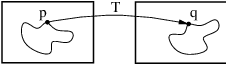
Figure 3.1: Image registration is the task of finding a spatial transform mapping one image into another.
Figure 3.1: Image registration is the task of finding a
spatial transform mapping one image into another.
This chapter introduces ITK’s capabilities for performing image registration. Image registration is the process of determining the spatial transform that maps points from one image to homologous points on a object in the second image. This concept is schematically represented in Figure 3.1. In ITK, registration is performed within a framework of pluggable components that can easily be interchanged. This flexibility means that a combinatorial variety of registration methods can be created, allowing users to pick and choose the right tools for their specific application.
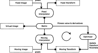
Let’s begin with a simplified typical registration framework where its components and their interconnections are shown in Figure 3.2. The basic input data to the registration process are two images: one is defined as the fixed image f(X) and the other as the moving image m(X), where X represents a position in N-dimensional space. Registration is treated as an optimization problem with the goal of finding the spatial mapping that will bring the moving image into alignment with the fixed image.
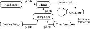
The transform component T (X) represents the spatial mapping of points from the fixed image space to points in the moving image space. The interpolator is used to evaluate moving image intensities at non-grid positions. The metric component S(f,m∘T ) provides a measure of how well the fixed image is matched by the transformed moving image. This measure forms a quantitative criterion to be optimized by the optimizer over the search space defined by the parameters of the transform.
ITKv4 registration framework provides more flexibility to the above traditional registration concept. In this new framework, the registration computations can happen on a physical grid completely different than the fixed image domain having different sampling density. This “sampling domain” is considered as a new component in the registration framework known as virtual image that can be an arbitrary set of physical points, not necessarily a uniform grid of points.
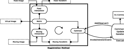
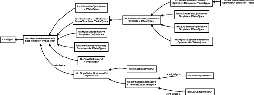
Various ITKv4 registration components are illustrated in Figure 3.3. Boxes with dashed borders show data objects, while those with solid borders show process objects.
The matching Metric class is a key component that controls most parts of the registration process since it handles fixed, moving and virtual images as well as fixed and moving transforms and interpolators.
Fixed and moving transforms and interpolators are used by the metric to evaluate the intensity values of the fixed and moving images at each physical point of the virtual space. Those intensity values are then used by the metric cost function to evaluate the fitness value and derivatives, which are passed to the optimizer that asks the moving transform to update its parameters based on the outputs of the cost function. Since the moving transform is shared between metric and optimizer, the above process will be repeated till the convergence criteria are met.
Later in section 3.3 you will get a better understanding of the behind-the-scenes processes of ITKv4 registration framework. First, we begin with some simple registration examples.
The source code for this section can be found in the file
ImageRegistration1.cxx.
This example illustrates the use of the image registration framework in Insight. It should be read as a “Hello World” for ITK registration. Instead of means to an end, this example should be read as a basic introduction to the elements typically involved when solving a problem of image registration.
A registration method requires the following set of components: two input images, a transform, a metric and an optimizer. Some of these components are parameterized by the image type for which the registration is intended. The following header files provide declarations of common types used for these components.
The type of each registration component should be instantiated first. We start by selecting the image dimension and the types to be used for representing image pixels.
The types of the input images are instantiated by the following lines.
The transform that will map the fixed image space into the moving image space is defined below.
An optimizer is required to explore the parameter space of the transform in search of optimal values of the metric.
The metric will compare how well the two images match each other. Metric types are usually templated over the image types as seen in the following type declaration.
The registration method type is instantiated using the types of the fixed and moving images as well as the output transform type. This class is responsible for interconnecting all the components that we have described so far.
Each one of the registration components is created using its New() method and is assigned to its respective itk::SmartPointer.
Each component is now connected to the instance of the registration method.
In this example the transform object does not need to be created and passed to the registration method like above since the registration filter will instantiate an internal transform object using the transform type that is passed to it as a template parameter.
Metric needs an interpolator to evaluate the intensities of the fixed and moving images at non-grid positions. The types of fixed and moving interpolators are declared here.
Then, fixed and moving interpolators are created and passed to the metric. Since linear interpolators are used as default, we could skip the following step in this example.
In this example, the fixed and moving images are read from files. This requires the itk::ImageRegistrationMethodv4 to acquire its inputs from the output of the readers.
Now the registration process should be initialized. ITKv4 registration framework provides initial transforms for both fixed and moving images. These transforms can be used to setup an initial known correction of the misalignment between the virtual domain and fixed/moving image spaces. In this particular case, a translation transform is being used for initialization of the moving image space. The array of parameters for the initial moving transform is simply composed of the translation values along each dimension. Setting the values of the parameters to zero initializes the transform to an Identity transform. Note that the array constructor requires the number of elements to be passed as an argument.
TransformType::Pointer movingInitialTransform = TransformType::New();
TransformType::ParametersType initialParameters(
movingInitialTransform->GetNumberOfParameters() );
initialParameters[0] = 0.0; // Initial offset in mm along X
initialParameters[1] = 0.0; // Initial offset in mm along Y
movingInitialTransform->SetParameters( initialParameters );
registration->SetMovingInitialTransform( movingInitialTransform );
In the registration filter this moving initial transform will be added to a composite transform that already includes an instantiation of the output optimizable transform; then, the resultant composite transform will be used by the optimizer to evaluate the metric values at each iteration.
Despite this, the fixed initial transform does not contribute to the optimization process. It is only used to access the fixed image from the virtual image space where the metric evaluation happens.
Virtual images are a new concept added to the ITKv4 registration framework, which potentially lets us to do the registration process in a physical domain totally different from the fixed and moving image domains. In fact, the region over which metric evaluation is performed is called virtual image domain. This domain defines the resolution at which the evaluation is performed, as well as the physical coordinate system.
The virtual reference domain is taken from the “virtual image” buffered region, and the input images should be accessed from this reference space using the fixed and moving initial transforms.
The legacy intuitive registration framework can be considered as a special case where the virtual domain is the same as the fixed image domain. As this case practically happens in most of the real life applications, the virtual image is set to be the same as the fixed image by default. However, the user can define the virtual domain differently than the fixed image domain by calling either SetVirtualDomain or SetVirtualDomainFromImage.
In this example, like the most examples of this chapter, the virtual image is considered the same as the fixed image. Since the registration process happens in the fixed image physical domain, the fixed initial transform maintains its default value of identity and does not need to be set.
However, a “Hello World!” example should show all the basics, so all the registration components are explicity set here.
In the next section of this chapter, you will get a better understanding from behind the scenes of the registration process when the initial fixed transform is not identity.
Note that the above process shows only one way of initializing the registration configuration. Another option is to initialize the output optimizable transform directly. In this approach, a transform object is created, initialized, and then passed to the registration method via SetInitialTransform(). This approach is shown in section 3.6.1.
At this point the registration method is ready for execution. The optimizer is the component that drives the execution of the registration. However, the ImageRegistrationMethodv4 class orchestrates the ensemble to make sure that everything is in place before control is passed to the optimizer.
It is usually desirable to fine tune the parameters of the optimizer. Each optimizer has particular parameters that must be interpreted in the context of the optimization strategy it implements. The optimizer used in this example is a variant of gradient descent that attempts to prevent it from taking steps that are too large. At each iteration, this optimizer will take a step along the direction of the itk::ImageToImageMetricv4 derivative. Each time the direction of the derivative abruptly changes, the optimizer assumes that a local extrema has been passed and reacts by reducing the step length by a relaxation factor. The reducing factor should have a value between 0 and 1. This factor is set to 0.5 by default, and it can be changed to a different value via SetRelaxationFactor(). Also, the default value for the initial step length is 1, and this value can be changed manually with the method SetLearningRate().
In addition to manual settings, the initial step size can also be estimated automatically, either at each iteration or only at the first iteration, by assigning a ScalesEstimator (as will be seen in later examples).
After several reductions of the step length, the optimizer may be moving in a very restricted area of the transform parameter space. By the method SetMinimumStepLength(), the user can define how small the step length should be to consider convergence to have been reached. This is equivalent to defining the precision with which the final transform should be known. User can also set some other stop criteria manually like maximum number of iterations.
In other gradient descent-based optimizers of the ITKv4 framework, such as itk::GradientDescentLineSearchOptimizerv4 and itk::ConjugateGradientLineSearchOptimizerv4, the convergence criteria are set via SetMinimumConvergenceValue() which is computed based on the results of the last few iterations. The number of iterations involved in computations are defined by the convergence window size via SetConvergenceWindowSize() which is shown in later examples of this chapter.
Also note that unlike the previous versions, ITKv4 optimizers do not have a “maximize/minimize” option to modify the effect of the metric derivatives. Each assigned metric is assumed to return a parameter derivative result that ”improves” the optimization.
In case the optimizer never succeeds reaching the desired precision tolerance, it is prudent to establish a limit on the number of iterations to be performed. This maximum number is defined with the method SetNumberOfIterations().
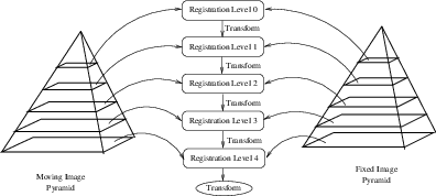
ITKv4 facilitates a multi-level registration framework whereby each stage is different in the resolution of its virtual space and the smoothness of the fixed and moving images. These criteria need to be defined before registration starts. Otherwise, the default values will be used. In this example, we run a simple registration in one level with no space shrinking or smoothing on the input data.
constexpr unsigned int numberOfLevels = 1;
RegistrationType::ShrinkFactorsArrayType shrinkFactorsPerLevel;
shrinkFactorsPerLevel.SetSize( 1 );
shrinkFactorsPerLevel[0] = 1;
RegistrationType::SmoothingSigmasArrayType smoothingSigmasPerLevel;
smoothingSigmasPerLevel.SetSize( 1 );
smoothingSigmasPerLevel[0] = 0;
registration->SetNumberOfLevels ( numberOfLevels );
registration->SetSmoothingSigmasPerLevel( smoothingSigmasPerLevel );
registration->SetShrinkFactorsPerLevel( shrinkFactorsPerLevel );
The registration process is triggered by an invocation of the Update() method. If something goes wrong during the initialization or execution of the registration an exception will be thrown. We should therefore place the Update() method inside a try/catch block as illustrated in the following lines.
In a real life application, you may attempt to recover from the error by taking more effective actions in the catch block. Here we are simply printing out a message and then terminating the execution of the program.
The result of the registration process is obtained using the GetTransform() method that returns a constant pointer to the output transform.
In the case of the itk::TranslationTransform, there is a straightforward interpretation of the parameters. Each element of the array corresponds to a translation along one spatial dimension.
The optimizer can be queried for the actual number of iterations performed to reach convergence. The GetCurrentIteration() method returns this value. A large number of iterations may be an indication that the learning rate has been set too small, which is undesirable since it results in long computational times.
The value of the image metric corresponding to the last set of parameters can be obtained with the GetValue() method of the optimizer.
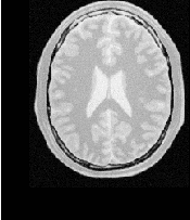
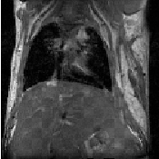
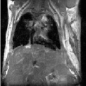
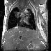
Let’s execute this example over two of the images provided in Examples/Data:
The second image is the result of intentionally translating the first image by (13,17) millimeters. Both images have unit-spacing and are shown in Figure 3.4. The registration takes 20 iterations and the resulting transform parameters are:
As expected, these values match quite well the misalignment that we intentionally introduced in the moving image.
It is common, as the last step of a registration task, to use the resulting transform to map the moving image into the fixed image space.
Before the mapping process, notice that we have not used the direct initialization of the output transform in this example, so the parameters of the moving initial transform are not reflected in the output parameters of the registration filter. Hence, a composite transform is needed to concatenate both initial and output transforms together.
using CompositeTransformType = itk::CompositeTransform<
double,
Dimension >;
CompositeTransformType::Pointer outputCompositeTransform =
CompositeTransformType::New();
outputCompositeTransform->AddTransform( movingInitialTransform );
outputCompositeTransform->AddTransform(
registration->GetModifiableTransform() );
Now the mapping process is easily done with the itk::ResampleImageFilter. Please refer to Section 2.9.4 for details on the use of this filter. First, a ResampleImageFilter type is instantiated using the image types. It is convenient to use the fixed image type as the output type since it is likely that the transformed moving image will be compared with the fixed image.
A resampling filter is created and the moving image is connected as its input.
The created output composite transform is also passed as input to the resampling filter.
As described in Section 2.9.4, the ResampleImageFilter requires additional parameters to be specified, in particular, the spacing, origin and size of the output image. The default pixel value is also set to a distinct gray level in order to highlight the regions that are mapped outside of the moving image.
FixedImageType::Pointer fixedImage = fixedImageReader->GetOutput();
resampler->SetSize( fixedImage->GetLargestPossibleRegion().GetSize() );
resampler->SetOutputOrigin( fixedImage->GetOrigin() );
resampler->SetOutputSpacing( fixedImage->GetSpacing() );
resampler->SetOutputDirection( fixedImage->GetDirection() );
resampler->SetDefaultPixelValue( 100 );
The output of the filter is passed to a writer that will store the image in a file. An itk::CastImageFilter is used to convert the pixel type of the resampled image to the final type used by the writer. The cast and writer filters are instantiated below.
The filters are created by invoking their New() method.
The filters are connected together and the Update() method of the writer is invoked in order to trigger the execution of the pipeline.
The fixed image and the transformed moving image can easily be compared using the itk::SubtractImageFilter. This pixel-wise filter computes the difference between homologous pixels of its two input images.
Note that the use of subtraction as a method for comparing the images is appropriate here because we chose to represent the images using a pixel type float. A different filter would have been used if the pixel type of the images were any of the unsigned integer types.
Since the differences between the two images may correspond to very low values of intensity, we rescale those intensities with a itk::RescaleIntensityImageFilter in order to make them more visible. This rescaling will also make it possible to visualize the negative values even if we save the difference image in a file format that only supports unsigned pixel values1 . We also reduce the DefaultPixelValue to “1” in order to prevent that value from absorbing the dynamic range of the differences between the two images.
using RescalerType = itk::RescaleIntensityImageFilter<
FixedImageType,
OutputImageType >;
RescalerType::Pointer intensityRescaler = RescalerType::New();
intensityRescaler->SetInput( difference->GetOutput() );
intensityRescaler->SetOutputMinimum( 0 );
intensityRescaler->SetOutputMaximum( 255 );
resampler->SetDefaultPixelValue( 1 );
Its output can be passed to another writer.
For the purpose of comparison, the difference between the fixed image and the moving image before registration can also be computed by simply setting the transform to an identity transform. Note that the resampling is still necessary because the moving image does not necessarily have the same spacing, origin and number of pixels as the fixed image. Therefore a pixel-by-pixel operation cannot in general be performed. The resampling process with an identity transform will ensure that we have a representation of the moving image in the grid of the fixed image.
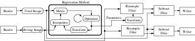
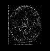
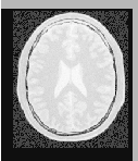
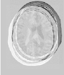
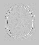
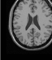
The complete pipeline structure of the current example is presented in Figure 3.6. The components of the registration method are depicted as well. Figure 3.5 (left) shows the result of resampling the moving image in order to map it onto the fixed image space. The top and right borders of the image appear in the gray level selected with the SetDefaultPixelValue() in the ResampleImageFilter. The center image shows the difference between the fixed image and the original moving image (i.e. the difference before the registration is performed). The right image shows the difference between the fixed image and the transformed moving image (i.e. after the registration has been performed). Both difference images have been rescaled in intensity in order to highlight those pixels where differences exist. Note that the final registration is still off by a fraction of a pixel, which causes bands around edges of anatomical structures to appear in the difference image. A perfect registration would have produced a null difference image.
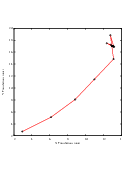
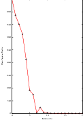
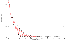
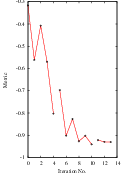
It is always useful to keep in mind that registration is essentially an optimization problem. Figure 3.7 helps to reinforce this notion by showing the trace of translations and values of the image metric at each iteration of the optimizer. It can be seen from the top figure that the step length is reduced progressively as the optimizer gets closer to the metric extrema. The bottom plot clearly shows how the metric value decreases as the optimization advances. The log plot helps to highlight the normal oscillations of the optimizer around the extrema value.
In this section, we used a very simple example to introduce the basic components of a registration process in ITKv4. However, studying this example alone is not enough to start using the itk::ImageRegistrationMethodv4. In order to choose the best registration practice for a specific application, knowledge of other registration method instantiations and their capabilities are required. For example, direct initialization of the output optimizable transform is shown in section 3.6.1. This method can simplify the registration process in many cases. Also, multi-resolution and multistage registration approaches are illustrated in sections 3.7 and 3.8. These examples illustrate the flexibility in the usage of ITKv4 registration method framework that can help to provide faster and more reliable registration processes.
This section presents internals of the registration process in ITKv4. Understanding what actually happens is necessary to have a correct interpretation of the results of a registration filter. It also helps to understand the most common difficulties that users encounter when they start using the ITKv4 registration framework:
These two topics tend to create confusion because they are implemented in different ways in other systems, and community members tend to have different expectations regarding how registration should work in ITKv4. The situation is further complicated by the way most people describe image operations, as if they were manually performed on a continuous picture on a piece of paper.
These concepts are discussed in this section through a general example shown in Figure 3.8.

Recall that ITKv4 does the registration in “physical” space where fixed, moving and virtual images are placed. Also, note that the term of virtual image is deceptive here since it does not refer to any actual image. In fact, the virtual image defines the origin, direction and the spacing of a space lattice that holds the output resampled image of the registration process. The virtual pixel lattice is illustrated in green at the top left side of Figure 3.8.
As shown in this figure, generally there are two transforms involved in the registration process even though only one of them is being optimized. T vm maps points from physical virtual space onto the physical space of the moving image, and in the same way T vf finds homologous points between physical virtual space and the physical space of the fixed image. Note that only T vm is optimized during the registration process. T vf cannot be optimized. The fixed transform usually is an identity transform since the virtual image lattice is commonly defined as the fixed image lattice.
When the registration starts, the algorithm goes through each grid point of the virtual lattice in a raster sweep. At each point the fixed and moving transforms find coordinates of the homologous points in the fixed and moving image physical spaces, and interpolators are used to find the pixel intensities if mapped points are in non-grid positions. These intensity values are passed to a cost function to find the current metric value.
Note the direction of the mapping transforms here. For example, if you consider the T vm transform, confusion often occurs since the transform shifts a virtual lattice point on the positive X direction. The visual effect of this mapping, once the moving image is resampled, is equivalent to manually shifting the moving image along the negative X direction. In the same way, when the T vm transform applies a clock-wise rotation to the virtual space points, the visual effect of this mapping, once the moving image has been resampled, is equivalent to manually rotating the moving image counter-clock-wise. The same relationships also occur with the T vf transform between the virtual space and the fixed image space.
This mapping direction is chosen because the moving image is resampled on the grid of the virtual image. In the resampling process, an algorithm iterates through every pixel of the output image and computes the intensity assigned to this pixel by mapping to its location in the moving image.
Instead, if we were to use the transform mapping coordinates from the moving image physical space into the virtual image physical space, then the resampling process would not guarantee that every pixel in the grid of the virtual image would receive one and only one value. In other words, the resampling would result in an image with holes and redundant or overlapping pixel values.
As seen in the previous examples, and as corroborated in the remaining examples in this chapter, the transform computed by the registration framework can be used directly in the resampling filter in order to map the moving image onto the discrete grid of the virtual image.
There are exceptional cases in which the transform desired is actually the inverse transform of the one computed by the ITK registration framework. Only those cases may require invoking the GetInverse() method that most transforms offer. Before attempting this, read the examples on resampling illustrated in section 2.9 in order to familiarize yourself with the correct interpretation of the transforms.
Now we come back to the situation illustrated in Figure 3.8. This figure shows the flexibility of the ITKv4 registration framework. We can register two images with different scales, sizes and resolutions. Also, we can create the output warped image with any desired size and resolution.
Nevertheless, note that the spatial transform computed during the registration process does not need to be concerned about a different number of pixels and different pixel sizes between fixed, moving and output images because the conversion from index space to the physical space implicitly takes care of the required scaling factor between the involved images.
One important consequence of this fact is that having the correct image origin, image pixel size, and image direction is fundamental for the success of the registration process in ITK, since we need this information to compute the exact location of each pixel lattice in the physical space; we must make sure that the correct values for the origin, spacing, and direction of all fixed, moving and virtual images are provided.
In this example, the spatial transform computed will physically map the brain from the moving image onto the virtual space and minimize its difference with the resampled brain from the fixed image into the virtual space. Fortunately in practice there is no need to resample the fixed image since the virtual image physical domain is often assumed to be the same as physical domain of the fixed image.
The source code for this section can be found in the file
ImageRegistration3.cxx.
Given the numerous parameters involved in tuning a registration method for a particular application, it is not uncommon for a registration process to run for several minutes and still produce a useless result. To avoid this situation it is quite helpful to track the evolution of the registration as it progresses. The following section illustrates the mechanisms provided in ITK for monitoring the activity of the ImageRegistrationMethodv4 class.
Insight implements the Observer/Command design pattern [20]. The classes involved in this implementation are the itk::Object, itk::Command and itk::EventObject classes. The Object is the base class of most ITK objects. This class maintains a linked list of pointers to event observers. The role of observers is played by the Command class. Observers register themselves with an Object, declaring that they are interested in receiving notification when a particular event happens. A set of events is represented by the hierarchy of the Event class. Typical events are Start, End, Progress and Iteration.
Registration is controlled by an itk::Optimizer, which generally executes an iterative process. Most Optimizer classes invoke an itk::IterationEvent at the end of each iteration. When an event is invoked by an object, this object goes through its list of registered observers (Commands) and checks whether any one of them has expressed interest in the current event type. Whenever such an observer is found, its corresponding Execute() method is invoked. In this context, Execute() methods should be considered callbacks. As such, some of the common sense rules of callbacks should be respected. For example, Execute() methods should not perform heavy computational tasks. They are expected to execute rapidly, for example, printing out a message or updating a value in a GUI.
The following code illustrates a simple way of creating a Observer/Command to monitor a registration process. This new class derives from the Command class and provides a specific implementation of the Execute() method. First, the header file of the Command class must be included.
Our custom command class is called CommandIterationUpdate. It derives from the Command class and declares for convenience the types Self and Superclass. This facilitates the use of standard macros later in the class implementation.
The following type alias declares the type of the SmartPointer capable of holding a reference to this object.
The itkNewMacro takes care of defining all the necessary code for the New() method. Those with curious minds are invited to see the details of the macro in the file itkMacro.h in the Insight/Code/Common directory.
In order to ensure that the New() method is used to instantiate the class (and not the C++ new operator), the constructor is declared protected.
Since this Command object will be observing the optimizer, the following type alias are useful for converting pointers when the Execute() method is invoked. Note the use of const on the declaration of OptimizerPointer. This is relevant since, in this case, the observer is not intending to modify the optimizer in any way. A const interface ensures that all operations invoked on the optimizer are read-only.
ITK enforces const-correctness. There is hence a distinction between the Execute() method that can be invoked from a const object and the one that can be invoked from a non-const object. In this particular example the non-const version simply invoke the const version. In a more elaborate situation the implementation of both Execute() methods could be quite different. For example, you could imagine a non-const interaction in which the observer decides to stop the optimizer in response to a divergent behavior. A similar case could happen when a user is controlling the registration process from a GUI.
Finally we get to the heart of the observer, the Execute() method. Two arguments are passed to this method. The first argument is the pointer to the object that invoked the event. The second argument is the event that was invoked.
Note that the first argument is a pointer to an Object even though the actual object invoking the event is probably a subclass of Object. In our case we know that the actual object is an optimizer. Thus we can perform a dynamic_cast to the real type of the object.
The next step is to verify that the event invoked is actually the one in which we are interested. This is checked using the RTTI2 support. The CheckEvent() method allows us to compare the actual type of two events. In this case we compare the type of the received event with an IterationEvent. The comparison will return true if event is of type IterationEvent or derives from IterationEvent. If we find that the event is not of the expected type then the Execute() method of this command observer should return without any further action.
If the event matches the type we are looking for, we are ready to query data from the optimizer. Here, for example, we get the current number of iterations, the current value of the cost function and the current position on the parameter space. All of these values are printed to the standard output. You could imagine more elaborate actions like updating a GUI or refreshing a visualization pipeline.
This concludes our implementation of a minimal Command class capable of observing our registration method. We can now move on to configuring the registration process.
Once all the registration components are in place we can create one instance of our observer. This is done with the standard New() method and assigned to a SmartPointer.
The newly created command is registered as observer on the optimizer, using the AddObserver() method. Note that the event type is provided as the first argument to this method. In order for the RTTI mechanism to work correctly, a newly created event of the desired type must be passed as the first argument. The second argument is simply the smart pointer to the observer. Figure 3.9 illustrates the interaction between the Command/Observer class and the registration method.
At this point, we are ready to execute the registration. The typical call to Update() will do it. Note again the use of the try/catch block around the Update() method in case an exception is thrown.
The registration process is applied to the following images in Examples/Data:
It produces the following output.
You can verify from the code in the Execute() method that the first column is the iteration number, the second column is the metric value and the third and fourth columns are the parameters of the transform, which is a 2D translation transform in this case. By tracking these values as the registration progresses, you will be able to determine whether the optimizer is advancing in the right direction and whether the step-length is reasonable or not. That will allow you to interrupt the registration process and fine-tune parameters without having to wait until the optimizer stops by itself.
Some of the most challenging cases of image registration arise when images of different modalities are involved. In such cases, metrics based on direct comparison of gray levels are not applicable. It has been extensively shown that metrics based on the evaluation of mutual information are well suited for overcoming the difficulties of multi-modality registration.
The concept of Mutual Information is derived from Information Theory and its application to image registration has been proposed in different forms by different groups [12, 37, 63]; a more detailed review can be found in [23, 46]. The Insight Toolkit currently provides two different implementations of Mutual Information metrics (see section 3.11 for details). The following example illustrates the practical use of one of these metrics.
The source code for this section can be found in the file
ImageRegistration4.cxx.
In this example, we will solve a simple multi-modality problem using an implementation of mutual information. This implementation was published by Mattes et. al [40].
First, we include the header files of the components used in this example.
In this example the image types and all registration components, except the metric, are declared as in Section 3.2. The Mattes mutual information metric type is instantiated using the image types.
The metric is created using the New() method and then connected to the registration object.
The metric requires the user to specify the number of bins used to compute the entropy. In a typical application, 50 histogram bins are sufficient. Note however, that the number of bins may have dramatic effects on the optimizer’s behavior.
To calculate the image gradients, an image gradient calculator based on ImageFunction is used instead of image gradient filters. Image gradient methods are defined in the superclass ImageToImageMetricv4.
Notice that in the ITKv4 registration framework, optimizers always try to minimize the cost function, and the metrics always return a parameter and derivative result that improves the optimization, so this metric computes the negative mutual information. The optimization parameters are tuned for this example, so they are not exactly the same as the parameters used in Section 3.2.
Note that large values of the learning rate will make the optimizer unstable. Small values, on the other hand, may result in the optimizer needing too many iterations in order to walk to the extrema of the cost function. The easy way of fine tuning this parameter is to start with small values, probably in the range of {1.0,5.0}. Once the other registration parameters have been tuned for producing convergence, you may want to revisit the learning rate and start increasing its value until you observe that the optimization becomes unstable. The ideal value for this parameter is the one that results in a minimum number of iterations while still keeping a stable path on the parametric space of the optimization. Keep in mind that this parameter is a multiplicative factor applied on the gradient of the metric. Therefore, its effect on the optimizer step length is proportional to the metric values themselves. Metrics with large values will require you to use smaller values for the learning rate in order to maintain a similar optimizer behavior.
Whenever the regular step gradient descent optimizer encounters change in the direction of movement in the parametric space, it reduces the size of the step length. The rate at which the step length is reduced is controlled by a relaxation factor. The default value of the factor is 0.5. This value, however may prove to be inadequate for noisy metrics since they tend to induce erratic movements on the optimizers and therefore result in many directional changes. In those conditions, the optimizer will rapidly shrink the step length while it is still too far from the location of the extrema in the cost function. In this example we set the relaxation factor to a number higher than the default in order to prevent the premature shrinkage of the step length.
Instead of using the whole virtual domain (usually fixed image domain) for the registration, we can use a spatial sampled point set by supplying an arbitrary point list over which to evaluate the metric. The point list is expected to be in the fixed image domain, and the points are transformed into the virtual domain internally as needed. The user can define the point set via SetFixedSampledPointSet(), and the point set is used by calling SetUsedFixedSampledPointSet().
Also, instead of dealing with the metric directly, the user may define the sampling percentage and sampling strategy for the registration framework at each level. In this case, the registration filter manages the sampling operation over the fixed image space based on the input strategy (REGULAR, RANDOM) and passes the sampled point set to the metric internally.
The number of spatial samples to be used depends on the content of the image. If the images are smooth and do not contain many details, the number of spatial samples can usually be as low as 1% of the total number of pixels in the fixed image. On the other hand, if the images are detailed, it may be necessary to use a much higher proportion, such as 20% to 50%. Increasing the number of samples improves the smoothness of the metric, and therefore helps when this metric is used in conjunction with optimizers that rely of the continuity of the metric values. The trade-off, of course, is that a larger number of samples results in longer computation times per every evaluation of the metric.
One mechanism for bringing the metric to its limit is to disable the sampling and use all the pixels present in the FixedImageRegion. This can be done with the SetUseSampledPointSet( false ) method. You may want to try this option only while you are fine tuning all other parameters of your registration. We don’t use this method in this current example though.
It has been demonstrated empirically that the number of samples is not a critical parameter for the registration process. When you start fine tuning your own registration process, you should start using high values of number of samples, for example in the range of 20% to 50% of the number of pixels in the fixed image. Once you have succeeded to register your images you can then reduce the number of samples progressively until you find a good compromise on the time it takes to compute one evaluation of the metric. Note that it is not useful to have very fast evaluations of the metric if the noise in their values results in more iterations being required by the optimizer to converge. You must then study the behavior of the metric values as the iterations progress, just as illustrated in section 3.4.
In ITKv4, a single virtual domain or spatial sample point set is used for the all iterations of the registration process. The use of a single sample set results in a smooth cost function that can improve the functionality of the optimizer.
The spatial point set is pseudo randomly generated. For reproducible results an integer seed should set.
Let’s execute this example over two of the images provided in Examples/Data:

The second image is the result of intentionally translating the image BrainProtonDensitySliceBorder20.png by (13,17) millimeters. Both images have unit-spacing and are shown in Figure 3.10. The registration process converges after 46 iterations and produces the following results:
These values are a very close match to the true misalignment introduced in the moving image.


The result of resampling the moving image is presented on the left of Figure 3.11. The center and right parts of the figure present a checkerboard composite of the fixed and moving images before and after registration respectively.
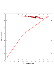
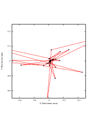
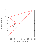
Figure 3.12 (upper-left) shows the sequence of translations followed by the optimizer as it searched the parameter space. The upper-right figure presents a closer look at the convergence basin for the last iterations of the optimizer. The bottom of the same figure shows the sequence of metric values computed as the optimizer searched the parameter space.
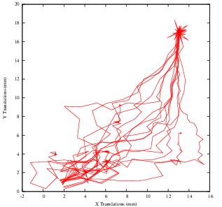
You must note however that there are a number of non-trivial issues involved in the fine tuning of parameters for the optimization. For example, the number of bins used in the estimation of Mutual Information has a dramatic effect on the performance of the optimizer. In order to illustrate this effect, the same example has been executed using a range of different values for the number of bins, from 10 to 30. If you repeat this experiment, you will notice that depending on the number of bins used, the optimizer’s path may get trapped early on in local minima. Figure 3.13 shows the multiple paths that the optimizer took in the parametric space of the transform as a result of different selections on the number of bins used by the Mattes Mutual Information metric. Note that many of the paths die in local minima instead of reaching the extrema value on the upper right corner.
Effects such as the one illustrated here highlight how useless is to compare different algorithms based on a non-exhaustive search of their parameter setting. It is quite difficult to be able to claim that a particular selection of parameters represent the best combination for running a particular algorithm. Therefore, when comparing the performance of two or more different algorithms, we are faced with the challenge of proving that none of the algorithms involved in the comparison are being run with a sub-optimal set of parameters.
The plots in Figures 3.12 and 3.13 were generated using Gnuplot3 . The scripts used for this purpose are available in the ITKSoftwareGuide Git repository under the directory
ITKSoftwareGuide/SoftwareGuide/Art.
Data for the plots were taken directly from the output that the Command/Observer in this example prints out to the console. The output was processed with the UNIX editor sed4 in order to remove commas and brackets that were confusing for Gnuplot’s parser. Both the shell script for running sed and for running Gnuplot are available in the directory indicated above. You may find useful to run them in order to verify the results presented here, and to eventually modify them for profiling your own registrations.
Open Science is not just an abstract concept. Open Science is something to be practiced every day with the simple gesture of sharing information with your peers, and by providing all the tools that they need for replicating the results that you are reporting. In Open Science, the only bad results are those that can not be replicated5 . Science is dead when people blindly trust authorities 6 instead of verifying their statements by performing their own experiments [47, 48].
The ITK image coordinate origin is typically located in one of the image corners (see the Defining Origin and Spacing section of Book 1 for details). This results in counter-intuitive transform behavior when rotations and scaling are involved. Users tend to assume that rotations and scaling are performed around a fixed point at the center of the image. In order to compensate for this difference in expected interpretation, the concept of center of transform has been introduced into the toolkit. This parameter is generally a fixed parameter that is not optimized during registration, so initialization is crucial to get efficient and accurate results. The following sections describe the main characteristics and effects of initializing the center of a transform.
The source code for this section can be found in the file
ImageRegistration5.cxx.
This example illustrates the use of the itk::Euler2DTransform for performing rigid registration in 2D. The example code is for the most part identical to that presented in Section 3.2. The main difference is the use of the Euler2DTransform here instead of the itk::TranslationTransform.
In addition to the headers included in previous examples, the following header must also be included.
The transform type is instantiated using the code below. The only template parameter for this class is the representation type of the space coordinates.
In the Hello World! example, we used Fixed/Moving initial transforms to initialize the registration configuration. That approach was good to get an intuition of the registration method, specifically when we aim to run a multistage registration process, from which the output of each stage can be used to initialize the next registration stage.
To get a better underestanding of the registration process in such situations, consider an example of 3 stages registration process that is started using an initial moving transform (Γmi). Multiple stages are handled by linking multiple instantiations of the itk::ImageRegistrationMethodv4 class. Inside the registration filter of the first stage, the initial moving transform is added to an internal composite transform along with an updatable identity transform (Γu). Although the whole composite transform is used for metric evaluation, only the Γu is set to be updated by the optimizer at each iteration. The Γu will be considered as the output transform of the current stage when the optimization process is converged. This implies that the output of this stage does not include the initialization parameters, so we need to concatenate the output and the initialization transform into a composite transform to be considered as the final transform of the first registration stage.
T 1(x) = Γmi(Γstage1(x))
Consider that, as explained in section 3.3, the above transform is a mapping from the vitual domain (i.e. fixed image space, when no fixed initial transform) to the moving image space.
Then, the result transform of the first stage will be used as the initial moving transform for the second stage of the registration process, and this approach goes on until the last stage of the registration process.
At the end of the registration process, the Γmi and the outputs of each stage can be concatenated into a final composite transform that is considered to be the final output of the whole registration process.
I′m(x) = Im(Γmi(Γstage1(Γstage2(Γstage3(x)))))
The above approach is especially useful if individual stages are characterized by different types of transforms, e.g. when we run a rigid registration process that is proceeded by an affine registration which is completed by a BSpline registration at the end.
In addition to the above method, there is also a direct initialization method in which the initial transform will be optimized directly. In this way the initial transform will be modified during the registration process, so it can be used as the final transform when the registration process is completed. This direct approach is conceptually close to what was happening in ITKv3 registration.
Using this method is very simple and efficient when we have only one level of registration, which is the case in this example. Also, a good application of this initialization method in a multi-stage scenario is when two consequent stages have the same transform types, or at least the initial parameters can easily be inferred from the result of the previous stage, such as when a translation transform is followed by a rigid transform.
The direct initialization approach is shown by the current example in which we try to initialize the parameters of the optimizable transform (Γu) directly.
For this purpose, first, the initial transform object is constructed below. This transform will be initialized, and its initial parameters will be used when the registration process starts.
In this example, the input images are taken from readers. The code below updates the readers in order to ensure that the image parameters (size, origin and spacing) are valid when used to initialize the transform. We intend to use the center of the fixed image as the rotation center and then use the vector between the fixed image center and the moving image center as the initial translation to be applied after the rotation.
The center of rotation is computed using the origin, size and spacing of the fixed image.
FixedImageType::Pointer fixedImage = fixedImageReader->GetOutput();
const SpacingType fixedSpacing = fixedImage->GetSpacing();
const OriginType fixedOrigin = fixedImage->GetOrigin();
const RegionType fixedRegion = fixedImage->GetLargestPossibleRegion();
const SizeType fixedSize = fixedRegion.GetSize();
TransformType::InputPointType centerFixed;
centerFixed[0] = fixedOrigin[0] + fixedSpacing[0] ⋆ fixedSize[0] / 2.0;
centerFixed[1] = fixedOrigin[1] + fixedSpacing[1] ⋆ fixedSize[1] / 2.0;
The center of the moving image is computed in a similar way.
MovingImageType::Pointer movingImage = movingImageReader->GetOutput();
const SpacingType movingSpacing = movingImage->GetSpacing();
const OriginType movingOrigin = movingImage->GetOrigin();
const RegionType movingRegion = movingImage->GetLargestPossibleRegion();
const SizeType movingSize = movingRegion.GetSize();
TransformType::InputPointType centerMoving;
centerMoving[0] = movingOrigin[0] + movingSpacing[0] ⋆ movingSize[0] / 2.0;
centerMoving[1] = movingOrigin[1] + movingSpacing[1] ⋆ movingSize[1] / 2.0;
Then, we initialize the transform by passing the center of the fixed image as the rotation center with the SetCenter() method. Also, the translation is set as the vector relating the center of the moving image to the center of the fixed image. This last vector is passed with the method SetTranslation().
Let’s finally initialize the rotation with a zero angle.
Now the current parameters of the initial transform will be set to a registration method, so they can be assigned to the Γu directly. Note that you should not confuse the following function with the SetMoving(Fixed)InitialTransform() methods that were used in Hello World! example.
Keep in mind that the scale of units in rotation and translation is quite different. For example, here we know that the first element of the parameters array corresponds to the angle that is measured in radians, while the other parameters correspond to the translations that are measured in millimeters, so a naive application of gradient descent optimizer will not produce a smooth change of parameters, because a similar change of δ to each parameter will produce a different magnitude of impact on the transform. As the result, we need “parameter scales” to customize the learning rate for each parameter. We can take advantage of the scaling functionality provided by the optimizers.
In this example we use small factors in the scales associated with translations. However, for the transforms with larger parameters sets, it is not intuitive for a user to set the scales. Fortunately, a framework for automated estimation of parameter scales is provided by ITKv4 that will be discussed later in the example of section 3.8.
using OptimizerScalesType = OptimizerType::ScalesType;
OptimizerScalesType optimizerScales(
initialTransform->GetNumberOfParameters() );
const double translationScale = 1.0 / 1000.0;
optimizerScales[0] = 1.0;
optimizerScales[1] = translationScale;
optimizerScales[2] = translationScale;
optimizer->SetScales( optimizerScales );
Next we set the normal parameters of the optimization method. In this case we are using an itk::RegularStepGradientDescentOptimizerv4. Below, we define the optimization parameters like the relaxation factor, learning rate (initial step length), minimal step length and number of iterations. These last two act as stopping criteria for the optimization.
Let’s execute this example over two of the images provided in Examples/Data:
The second image is the result of intentionally rotating the first image by 10 degrees around the geometrical center of the image. Both images have unit-spacing and are shown in Figure 3.14. The registration takes 17 iterations and produces the results:
These results are interpreted as
As expected, these values match the misalignment intentionally introduced into the moving image quite well, since 10 degrees is about 0.174532 radians.

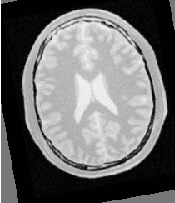
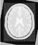
Figure 3.15 shows from left to right the resampled moving image after registration, the difference between the fixed and moving images before registration, and the difference between the fixed and resampled moving image after registration. It can be seen from the last difference image that the rotational component has been solved but that a small centering misalignment persists.
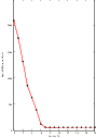
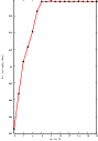
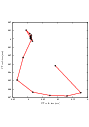
Figure 3.16 shows plots of the main output parameters produced from the registration process. This includes the metric values at every iteration, the angle values at every iteration, and the translation components of the transform as the registration progresses.
Let’s now consider the case in which rotations and translations are present in the initial registration, as in the following pair of images:
The second image is the result of intentionally rotating the first image by 10 degrees and then translating it 13mm in X and 17mm in Y . Both images have unit-spacing and are shown in Figure 3.17. In order to accelerate convergence it is convenient to use a larger step length as shown here.
optimizer->SetMaximumStepLength( 1.3 );
The registration now takes 37 iterations and produces the following results:
These parameters are interpreted as
These values approximately match the initial misalignment intentionally introduced into the moving image, since 10 degrees is about 0.174532 radians. The horizontal translation is well resolved while the vertical translation ends up being off by about one millimeter.
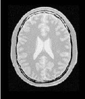


Figure 3.18 shows the output of the registration. The rightmost image of this figure shows the difference between the fixed image and the resampled moving image after registration.
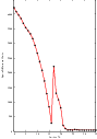
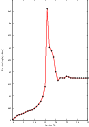
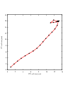
Figure 3.19 shows plots of the main output registration parameters when the rotation and translations are combined. These results include the metric values at every iteration, the angle values at every iteration, and the translation components of the registration as the registration converges. It can be seen from the smoothness of these plots that a larger step length could have been supported easily by the optimizer. You may want to modify this value in order to get a better idea of how to tune the parameters.
The source code for this section can be found in the file
ImageRegistration6.cxx.
This example illustrates the use of the itk::Euler2DTransform for performing registration. The example code is for the most part identical to the one presented in Section 3.6.1. Even though this current example is done in 2D, the class itk::CenteredTransformInitializer is quite generic and could be used in other dimensions. The objective of the initializer class is to simplify the computation of the center of rotation and the translation required to initialize certain transforms such as the Euler2DTransform. The initializer accepts two images and a transform as inputs. The images are considered to be the fixed and moving images of the registration problem, while the transform is the one used to register the images.
The CenteredTransformInitializer supports two modes of operation. In the first mode, the centers of the images are computed as space coordinates using the image origin, size and spacing. The center of the fixed image is assigned as the rotational center of the transform while the vector going from the fixed image center to the moving image center is passed as the initial translation of the transform. In the second mode, the image centers are not computed geometrically but by using the moments of the intensity gray levels. The center of mass of each image is computed using the helper class itk::ImageMomentsCalculator. The center of mass of the fixed image is passed as the rotational center of the transform while the vector going from the fixed image center of mass to the moving image center of mass is passed as the initial translation of the transform. This second mode of operation is quite convenient when the anatomical structures of interest are not centered in the image. In such cases the alignment of the centers of mass provides a better rough initial registration than the simple use of the geometrical centers. The validity of the initial registration should be questioned when the two images are acquired in different imaging modalities. In those cases, the center of mass of intensities in one modality does not necessarily match the center of mass of intensities in the other imaging modality.
The following are the most relevant headers in this example.
The transform type is instantiated using the code below. The only template parameter of this class is the representation type of the space coordinates.
Like the previous section, a direct initialization method is used here. The transform object is constructed below. This transform will be initialized, and its initial parameters will be considered as the parameters to be used when the registration process begins.
The input images are taken from readers. It is not necessary to explicitly call Update() on the readers since the CenteredTransformInitializer class will do it as part of its initialization. The following code instantiates the initializer. This class is templated over the fixed and moving images type as well as the transform type. An initializer is then constructed by calling the New() method and assigning the result to a itk::SmartPointer.
The initializer is now connected to the transform and to the fixed and moving images.
The use of the geometrical centers is selected by calling GeometryOn() while the use of center of mass is selected by calling MomentsOn(). Below we select the center of mass mode.
Finally, the computation of the center and translation is triggered by the InitializeTransform() method. The resulting values will be passed directly to the transform.
The remaining parameters of the transform are initialized as before.
Now the initialized transform object will be set to the registration method, and the starting point of the registration is defined by its initial parameters.
If the InPlaceOn() method is called, this initialized transform will be the output transform object or “grafted” to the output. Otherwise, this “InitialTransform” will be deep-copied or “cloned” to the output.
Since the registration filter has InPlace set, the transform object is grafted to the output and is updated by the registration method.
Let’s execute this example over some of the images provided in Examples/Data, for example:
The second image is the result of intentionally rotating the first image by 10 degrees around the geometric center and shifting it 13mm in X and 17mm in Y . Both images have unit-spacing and are shown in Figure 3.14. The registration takes 21 iterations and produces:
These parameters are interpreted as
Note that the reported translation is not the translation of (13,17) that might be expected. The reason is that we used the center of mass (111.204,131.591) for the fixed center, while the input was rotated about the geometric center (110.5,128.5). It is more illustrative in this case to take a look at the actual rotation matrix and offset resulting from the five parameters.
Which produces the following output.
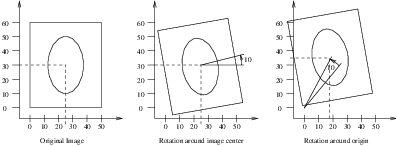
This output illustrates how counter-intuitive the mix of center of rotation and translations can be. Figure 3.20 will clarify this situation. The figure shows the original image on the left. A rotation of 10∘ around the center of the image is shown in the middle. The same rotation performed around the origin of coordinates is shown on the right. It can be seen here that changing the center of rotation introduces additional translations.
Let’s analyze what happens to the center of the image that we just registered. Under the point of view of rotating 10∘ around the center and then applying a translation of (13mm,17mm). The image has a size of (221×257) pixels and unit spacing. Hence its center has coordinates (110.5,128.5). Since the rotation is done around this point, the center behaves as the fixed point of the transformation and remains unchanged. Then with the (13mm,17mm) translation it is mapped to (123.5,145.5) which becomes its final position.
The matrix and offset that we obtained at the end of the registration indicate that this should be equivalent to a rotation of 10∘ around the origin, followed by a translation of (36.99,-1.23). Let’s compute this in detail. First the rotation of the image center by 10∘ around the origin will move the point (110.5,128.5) to (86.51,145.74). Now, applying a translation of (36.99,-1.23) maps this point to (123.50,144.50), which is very close to the result of our previous computation.
It is unlikely that we could have chosen these translations as the initial guess, since we tend to think about images in a coordinate system whose origin is in the center of the image.
This underscores the importance of using good initialization for the center for a transform fixed parameter. By using either the center of geometry or center of mass for initialization the rotation and translation parameters may have a more intuitive interpretation than if only the optimization parameters of translation and rotation are initialized.


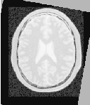

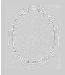
Figure 3.22 shows the output of the registration. The image on the right of this figure shows the differences between the fixed image and the resampled moving image after registration.
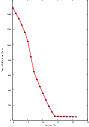
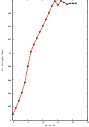
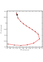
Figure 3.23 plots the output parameters of the registration process. It includes the metric values at every iteration, the angle values at every iteration, and the values of the translation components as the registration progresses. Note that this is the complementary translation as used in the transform, not the actual total translation that is used in the transform offset. We could modify the observer to print the total offset instead of printing the array of parameters. Let’s call that an exercise for the reader!
The source code for this section can be found in the file
ImageRegistration7.cxx.
This example illustrates the use of the itk::Simularity2DTransform class for performing registration in 2D. The example code is for the most part identical to the code presented in Section 3.6.2. The main difference is the use of itk::Simularity2DTransform here rather than the itk::Euler2DTransform class.
A similarity transform can be seen as a composition of rotations, translations and uniform  scaling. It preserves angles and maps lines into lines. This transform is implemented in the toolkit as
deriving from a rigid 2D transform and with a scale parameter added.
scaling. It preserves angles and maps lines into lines. This transform is implemented in the toolkit as
deriving from a rigid 2D transform and with a scale parameter added.
When using this transform, attention should be paid to the fact that scaling and translations are not independent. In the same way that rotations can locally be seen as translations, scaling also results in local displacements. Scaling is performed in general with respect to the origin of coordinates. However, we already saw how ambiguous that could be in the case of rotations. For this reason, this transform also allows users to setup a specific center. This center is used both for rotation and scaling.
In addition to the headers included in previous examples, here the following header must be included.
The Transform class is instantiated using the code below. The only template parameter of this class is the representation type of the space coordinates.
As before, the transform object is constructed and initialized before it is passed to the registration filter.
In this example, we again use the helper class itk::CenteredTransformInitializer to compute a reasonable value for the initial center of rotation and scaling along with an initial translation.
using TransformInitializerType = itk::CenteredTransformInitializer<
TransformType,
FixedImageType,
MovingImageType >;
TransformInitializerType::Pointer initializer
= TransformInitializerType::New();
initializer->SetTransform( transform );
initializer->SetFixedImage( fixedImageReader->GetOutput() );
initializer->SetMovingImage( movingImageReader->GetOutput() );
initializer->MomentsOn();
initializer->InitializeTransform();
The remaining parameters of the transform are initialized below.
Now the initialized transform object will be set to the registration method, and its initial parameters are used to initialize the registration process.
Also, by calling the InPlaceOn() method, this initialized transform will be the output transform object or “grafted” to the output of the registration process.
Keeping in mind that the scale of units in scaling, rotation and translation are quite different, we take advantage of the scaling functionality provided by the optimizers. We know that the first element of the parameters array corresponds to the scale factor, the second corresponds to the angle, third and fourth are the remaining translation. We use henceforth small factors in the scales associated with translations.
using OptimizerScalesType = OptimizerType::ScalesType;
OptimizerScalesType optimizerScales( transform->GetNumberOfParameters() );
const double translationScale = 1.0 / 100.0;
optimizerScales[0] = 10.0;
optimizerScales[1] = 1.0;
optimizerScales[2] = translationScale;
optimizerScales[3] = translationScale;
optimizer->SetScales( optimizerScales );
We also set the ordinary parameters of the optimization method. In this case we are using a itk::RegularStepGradientDescentOptimizerv4. Below we define the optimization parameters, i.e. initial learning rate (step length), minimal step length and number of iterations. The last two act as stopping criteria for the optimization.
Let’s execute this example over some of the images provided in Examples/Data, for example:
The second image is the result of intentionally rotating the first image by 10 degrees, scaling by 1∕1.2 and then translating by (-13,-17). Both images have unit-spacing and are shown in Figure 3.24. The registration takes 53 iterations and produces:
That are interpreted as
These values approximate the misalignment intentionally introduced into the moving image. Since 10 degrees is about 0.174532 radians.

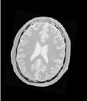
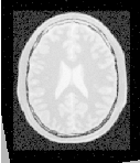
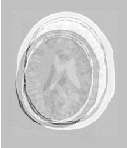
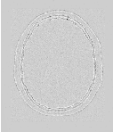
Figure 3.25 shows the output of the registration. The right image shows the squared magnitude of pixel differences between the fixed image and the resampled moving image.
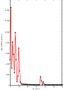
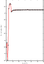
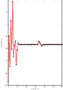
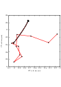
Figure 3.26 shows the plots of the main output parameters of the registration process. The metric values at every iteration are shown on the left. The rotation angle and scale factor values are shown in the two center plots while the translation components of the registration are presented in the plot on the right.
The source code for this section can be found in the file
ImageRegistration8.cxx.
This example illustrates the use of the itk::VersorRigid3DTransform class for performing registration of two 3D images. The class itk::CenteredTransformInitializer is used to initialize the center and translation of the transform. The case of rigid registration of 3D images is probably one of the most common uses of image registration.
The following are the most relevant headers of this example.
The parameter space of the VersorRigid3DTransform is not a vector space, because addition is not a closed operation in the space of versor components. Hence, we need to use Versor composition operation to update the first three components of the parameter array (rotation parameters), and Vector addition for updating the last three components of the parameters array (translation parameters) [24, 27].
In the previous version of ITK, a special optimizer, itk::VersorRigid3DTransformOptimizer was needed for registration to deal with versor computations. Fortunately in ITKv4, the itk::RegularStepGradientDescentOptimizerv4 can be used for both vector and versor transform optimizations because, in the new registration framework, the task of updating parameters is delegated to the moving transform itself. The UpdateTransformParameters method is implemented in the itk::Transform class as a virtual function, and all the derived transform classes can have their own implementations of this function. Due to this fact, the updating function is re-implemented for versor transforms so it can handle versor composition of the rotation parameters.
The Transform class is instantiated using the code below. The only template parameter to this class is the representation type of the space coordinates.
The initial transform object is constructed below. This transform will be initialized, and its initial parameters will be used when the registration process starts.
The input images are taken from readers. It is not necessary here to explicitly call Update() on the readers since the itk::CenteredTransformInitializer will do it as part of its computations. The following code instantiates the type of the initializer. This class is templated over the fixed and moving image types as well as the transform type. An initializer is then constructed by calling the New() method and assigning the result to a smart pointer.
The initializer is now connected to the transform and to the fixed and moving images.
The use of the geometrical centers is selected by calling GeometryOn() while the use of center of mass is selected by calling MomentsOn(). Below we select the center of mass mode.
Finally, the computation of the center and translation is triggered by the InitializeTransform() method. The resulting values will be passed directly to the transform.
The rotation part of the transform is initialized using a itk::Versor which is simply a unit quaternion. The VersorType can be obtained from the transform traits. The versor itself defines the type of the vector used to indicate the rotation axis. This trait can be extracted as VectorType. The following lines create a versor object and initialize its parameters by passing a rotation axis and an angle.
Now the current initialized transform will be set to the registration method, so its initial parameters can be used to initialize the registration process.
Let’s execute this example over some of the images available in the following website
http://public.kitware.com/pub/itk/Data/BrainWeb.
Note that the images in this website are compressed in .tgz files. You should download these files and decompress them in your local system. After decompressing and extracting the files you could take a pair of volumes, for example the pair:
The second image is the result of intentionally rotating the first image by 10 degrees around the origin and shifting it 15mm in X.
Also, instead of doing the above steps manually, you can turn on the following flag in your build environment:
ITK_USE_BRAINWEB_DATA
Then, the above data will be loaded to your local ITK build directory.
The registration takes 21 iterations and produces:
That are interpreted as
This Versor is equivalent to a rotation of 9.98 degrees around the Z axis.
Note that the reported translation is not the translation of (15.0,0.0,0.0) that we may be naively expecting. The reason is that the VersorRigid3DTransform is applying the rotation around the center found by the CenteredTransformInitializer and then adding the translation vector shown above.
It is more illustrative in this case to take a look at the actual rotation matrix and offset resulting from the 6 parameters.
The output of this print statements is
From the rotation matrix it is possible to deduce that the rotation is happening in the X,Y plane and that the angle is on the order of arcsin(0.173769) which is very close to 10 degrees, as we expected.


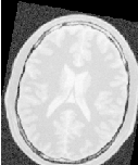
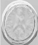
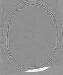
Figure 3.28 shows the output of the registration. The center image in this figure shows the differences between the fixed image and the resampled moving image before the registration. The image on the right side presents the difference between the fixed image and the resampled moving image after the registration has been performed. Note that these images are individual slices extracted from the actual volumes. For details, look at the source code of this example, where the ExtractImageFilter is used to extract a slice from the the center of each one of the volumes. One of the main purposes of this example is to illustrate that the toolkit can perform registration on images of any dimension. The only limitations are, as usual, the amount of memory available for the images and the amount of computation time that it will take to complete the optimization process.
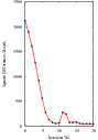
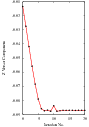
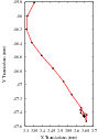
Figure 3.29 shows the plots of the main output parameters of the registration process. The Z component of the versor is plotted as an indication of how the rotation progresses. The X,Y translation components of the registration are plotted at every iteration too.
Shell and Gnuplot scripts for generating the diagrams in Figure 3.29 are available in the ITKSoftwareGuide Git repository under the directory
ITKSoftwareGuide/SoftwareGuide/Art.
You are strongly encouraged to run the example code, since only in this way can you gain first-hand experience with the behavior of the registration process. Once again, this is a simple reflection of the philosophy that we put forward in this book:
If you can not replicate it, then it does not exist!
We have seen enough published papers with pretty pictures, presenting results that in practice are impossible to replicate. That is vanity, not science.
The source code for this section can be found in the file
ImageRegistration9.cxx.
This example illustrates the use of the itk::AffineTransform for performing registration in 2D. The example code is, for the most part, identical to that in 3.6.2. The main difference is the use of the AffineTransform here instead of the itk::Euler2DTransform. We will focus on the most relevant changes in the current code and skip the basic elements already explained in previous examples.
Let’s start by including the header file of the AffineTransform.
We then define the types of the images to be registered.
The transform type is instantiated using the code below. The template parameters of this class are the representation type of the space coordinates and the space dimension.
The transform object is constructed below and is initialized before the registration process starts.
In this example, we again use the itk::CenteredTransformInitializer helper class in order to compute reasonable values for the initial center of rotation and the translations. The initializer is set to use the center of mass of each image as the initial correspondence correction.
using TransformInitializerType = itk::CenteredTransformInitializer<
TransformType,
FixedImageType,
MovingImageType >;
TransformInitializerType::Pointer initializer
= TransformInitializerType::New();
initializer->SetTransform( transform );
initializer->SetFixedImage( fixedImageReader->GetOutput() );
initializer->SetMovingImage( movingImageReader->GetOutput() );
initializer->MomentsOn();
initializer->InitializeTransform();
Now we pass the transform object to the registration filter, and it will be grafted to the output transform of the registration filter by updating its parameters during the the registration process.
Keeping in mind that the scale of units in scaling, rotation and translation are quite different, we take advantage of the scaling functionality provided by the optimizers. We know that the first N ×N elements of the parameters array correspond to the rotation matrix factor, and the last N are the components of the translation to be applied after multiplication with the matrix is performed.
using OptimizerScalesType = OptimizerType::ScalesType;
OptimizerScalesType optimizerScales( transform->GetNumberOfParameters() );
optimizerScales[0] = 1.0;
optimizerScales[1] = 1.0;
optimizerScales[2] = 1.0;
optimizerScales[3] = 1.0;
optimizerScales[4] = translationScale;
optimizerScales[5] = translationScale;
optimizer->SetScales( optimizerScales );
We also set the usual parameters of the optimization method. In this case we are using an itk::RegularStepGradientDescentOptimizerv4 as before. Below, we define the optimization parameters like learning rate (initial step length), minimum step length and number of iterations. These last two act as stopping criteria for the optimization.
Finally we trigger the execution of the registration method by calling the Update() method. The call is placed in a try/catch block in the case any exceptions are thrown.
Once the optimization converges, we recover the parameters from the registration method. We can also recover the final value of the metric with the GetValue() method and the final number of iterations with the GetCurrentIteration() method.
const TransformType::ParametersType finalParameters =
registration->GetOutput()->Get()->GetParameters();
const double finalRotationCenterX = transform->GetCenter()[0];
const double finalRotationCenterY = transform->GetCenter()[1];
const double finalTranslationX = finalParameters[4];
const double finalTranslationY = finalParameters[5];
const unsigned int numberOfIterations = optimizer->GetCurrentIteration();
const double bestValue = optimizer->GetValue();
Let’s execute this example over two of the images provided in Examples/Data:
The second image is the result of intentionally rotating the first image by 10 degrees and then translating by (-13,-17). Both images have unit-spacing and are shown in Figure 3.30. We execute the code using the following parameters: step length=1.0, translation scale= 0.0001 and maximum number of iterations = 300. With these images and parameters the registration takes 92 iterations and produces
These results are interpreted as
The second component of the matrix values is usually associated with sinθ. We obtain the rotation through SVD of the affine matrix. The value is 9.9494 degrees, which is approximately the intentional misalignment of 10.0 degrees.

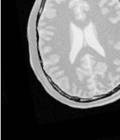

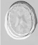
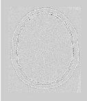
Figure 3.31 shows the output of the registration. The right most image of this figure shows the squared magnitude difference between the fixed image and the resampled moving image.
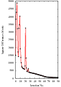
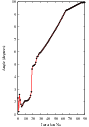
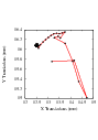
Figure 3.32 shows the plots of the main output parameters of the registration process. The metric values at every iteration are shown on the left plot. The angle values are shown on the middle plot, while the translation components of the registration are presented on the right plot. Note that the final total offset of the transform is to be computed as a combination of the shift due to rotation plus the explicit translation set on the transform.
Performing image registration using a multi-resolution approach is widely used to improve speed, accuracy and robustness. The basic idea is that registration is first performed at a coarse scale where the images have fewer pixels. The spatial mapping determined at the coarse level is then used to initialize registration at the next finer scale. This process is repeated until it reaches the finest possible scale. This coarse-to-fine strategy greatly improves the registration success rate and also increases robustness by eliminating local optima at coarser scales. Robustness can be improved even more by smoothing the images at coarse scales.
In all previous examples we ran the registration process at a single resolution. However, the ITKv4 registration framework is structured to provide a multi-resolution registration method. For this purpose we only need to define the number of levels as well as the resolution and smoothness of the input images at each level. The registration filter smoothes and subsamples the images according to user-defined ShrinkFactor and SmoothingSigma vectors.
We now present the multi-resolution capabilities of the framework by way of an example.
In ITK, the itk::MultiResolutionPyramidImageFilter can be used to create a sequence of reduced resolution images from the input image. The down-sampling is performed according to a user defined multi-resolution schedule. The schedule is specified as an itk::Array2D of integers, containing shrink factors for each multi-resolution level (rows) for each dimension (columns). For example,
is a schedule for a three dimensional image for two multi-resolution levels. In the first (coarsest) level, the image is reduced by a factor of 8 in the column dimension, factor of 4 in the row dimension and a factor of 4 in the slice dimension. In the second level, the image reduced by a factor of 4 in the column dimension, 4 in the row dimension and 2 in the slice dimension.
The method SetNumberOfLevels() is used to set the number of resolution levels in the pyramid. This method will allocate memory for the schedule and generate a default table with the starting (coarsest) shrink factors for all dimensions set to 2(M-1), where M is the number of levels. All factors are halved for all subsequent levels. For example, if we set the number of levels to 4, the default schedule is then:
The user can get a copy of the schedule using method GetSchedule(), make modifications, and reset it using method SetSchedule(). Alternatively, a user can create a default table by specifying the starting (coarsest) shrink factors using the method SetStartingShrinkFactors(). The factors for the subsequent levels are generated by halving the factor or setting it to one, depending on which is larger. For example, for a 4 level pyramid and starting factors of 8, 8 and 4, the generated schedule would be:
When this filter is triggered by Update(), M outputs are produced where the m-th output corresponds to the m-th level of the pyramid. To generate these images, Gaussian smoothing is first performed using a itk::DiscreteGaussianImageFilter with the variance set to (s∕2)2, where s is the shrink factor. The smoothed images are then sub-sampled using a itk::ShrinkImageFilter.
The source code for this section can be found in the file
MultiResImageRegistration1.cxx.
This example illustrates the use of the itk::ImageRegistrationMethodv4 to solve a simple multi-modality registration problem by a multi-resolution approach. Since ITKv4 registration method is designed based on a multi-resolution structure, a separate set of classes are no longer required to run the registration process of this example.
This a great advantage over the previous versions of ITK, as in ITKv3 we had to use a different filter ( itk::MultiResolutionImageRegistrationMethod) to run a multi-resolution process. Also, we had to use image pyramids filters ( itk::MultiResolutionPyramidImageFilter) for creating the sequence of downsampled images. Hence, you can see how ITKv4 framework is more user-friendly in more complex situations.
To begin the example, we include the headers of the registration components we will use.
The ImageRegistrationMethodv4 solves a registration problem in a coarse-to-fine manner as illustrated in Figure 3.33. The registration is first performed at the coarsest level using the images at the first level of the fixed and moving image pyramids. The transform parameters determined by the registration are then used to initialize the registration at the next finer level using images from the second level of the pyramids. This process is repeated as we work up to the finest level of image resolution.
In a typical registration scenario, a user will tweak component settings or even swap out components between multi-resolution levels. For example, when optimizing at a coarse resolution, it may be possible to take more aggressive step sizes and have a more relaxed convergence criterion.
Tweaking the components between resolution levels can be done using ITK’s implementation of the Command/Observer design pattern. Before beginning registration at each resolution level, where ImageRegistrationMethodv4 invokes a MultiResolutionIterationEvent(). The registration components can be changed by implementing a itk::Command which responds to the event. A brief description of the interaction between events and commands was previously presented in Section 3.4.
We will illustrate this mechanism by changing the parameters of the optimizer between each resolution level by way of a simple interface command. First, we include the header file of the Command class.
Our new interface command class is called RegistrationInterfaceCommand. It derives from Command and is templated over the multi-resolution registration type.
We then define Self, Superclass, Pointer, New() and a constructor in a similar fashion to the CommandIterationUpdate class in Section 3.4.
For convenience, we declare types useful for converting pointers in the Execute() method.
Two arguments are passed to the Execute() method: the first is the pointer to the object which invoked the event and the second is the event that was invoked.
First we verify that the event invoked is of the right type, itk::MultiResolutionIterationEvent(). If not, we return without any further action.
We then convert the input object pointer to a RegistrationPointer. Note that no error checking is done here to verify the dynamic_cast was successful since we know the actual object is a registration method. Then we ask for the optimizer object from the registration method.
If this is the first resolution level we set the learning rate (representing the first step size) and the minimum step length (representing the convergence criterion) to large values. At each subsequent resolution level, we will reduce the minimum step length by a factor of 5 in order to allow the optimizer to focus on progressively smaller regions. The learning rate is set up to the current step length. In this way, when the optimizer is reinitialized at the beginning of the registration process for the next level, the step length will simply start with the last value used for the previous level. This will guarantee the continuity of the path taken by the optimizer through the parameter space.
Another version of the Execute() method accepting a const input object is also required since this method is defined as pure virtual in the base class. This version simply returns without taking any action.
The fixed and moving image types are defined as in previous examples. The downsampled images for different resolution levels are created internally by the registration method based on the values provided for ShrinkFactor and SmoothingSigma vectors.
The types for the registration components are then derived using the fixed and moving image type, as in previous examples.
To set the optimizer parameters, note that LearningRate and MinimumStepLength are set in the obsever at the begining of each resolution level. The other optimizer parameters are set as follows.
We set the number of multi-resolution levels to three and set the corresponding shrink factor and smoothing sigma values for each resolution level. Using smoothing in the subsampled images in low-resolution levels can avoid large fluctuations in the metric function, which prevents the optimizer from becoming trapped in local minima. In this simple example we have no smoothing, and we have used small shrinkings for the first two resolution levels.
constexpr unsigned int numberOfLevels = 3;
RegistrationType::ShrinkFactorsArrayType shrinkFactorsPerLevel;
shrinkFactorsPerLevel.SetSize( 3 );
shrinkFactorsPerLevel[0] = 3;
shrinkFactorsPerLevel[1] = 2;
shrinkFactorsPerLevel[2] = 1;
RegistrationType::SmoothingSigmasArrayType smoothingSigmasPerLevel;
smoothingSigmasPerLevel.SetSize( 3 );
smoothingSigmasPerLevel[0] = 0;
smoothingSigmasPerLevel[1] = 0;
smoothingSigmasPerLevel[2] = 0;
registration->SetNumberOfLevels ( numberOfLevels );
registration->SetShrinkFactorsPerLevel( shrinkFactorsPerLevel );
registration->SetSmoothingSigmasPerLevel( smoothingSigmasPerLevel );
Once all the registration components are in place we can create an instance of our interface command and connect it to the registration object using the AddObserver() method.
Then we trigger the registration process by calling Update().
Let’s execute this example using the following images
The output produced by the execution of the method is
These values are a close match to the true misalignment of (13,17) introduced in the moving image.
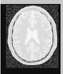
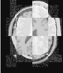
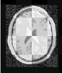
The result of resampling the moving image is presented in the left image of Figure 3.34. The center and right images of the figure depict a checkerboard composite of the fixed and moving images before and after registration.
Figure 3.35 (left) shows the sequence of translations followed by the optimizer as it searched the parameter space. The right side of the same figure shows the sequence of metric values computed as the optimizer searched the parameter space. From the trace, we can see that with the more aggressive optimization parameters we get quite close to the optimal value within 5 iterations with the remaining iterations just doing fine adjustments. It is interesting to compare these results with those of the single resolution example in Section 3.5.1, where 46 iterations were required as more conservative optimization parameters had to be used.
In section 3.7 you noticed how to tweak component settings between multi-resolution levels and saw how it can benefit the registration process. That is, the matching metric gets close to the optimal value before final parameter adjustments in full resolution. This approach saves large amounts of time in most practical cases, since fewer iterations are required at the full resolution level. This is helpful in cases like a deformable registration process on a large dataset, e.g. a high-resolution 3D image.
Another possible scheme is to apply a simple rigid transform for the initial coarse registration, then upgrade to an affine transform at the finer level. Finally, proceed to a deformable transform at the last level when we are close enough to the optimal value.
Fortunately, itk::ImageRegistrationMethodv4 allows for multistage registration whereby each stage is characterized by possibly different transforms and different image metrics. As in the above situation, you may want to perform a linear registration followed by a deformable registration with both stages performed across multiple resolutions.
Multiple stages are handled by linking multiple instantiations of this class. An optional composite transform can be used as a container to concatenate the output transforms of multiple stages.
We now present the multistage capabilities of the framework by way of an example.
The source code for this section can be found in the file
MultiStageImageRegistration1.cxx.
This example illustrates the use of more complex components of the registration framework. In particular, it introduces a multistage, multi-resolution approach to run a multi-modal registration process using two linear itk::TranslationTransform and itk::AffineTransform. Also, it shows the use of Scale Estimators for fine-tuning the scale parameters of the optimizer when an Affine transform is used. The itk::RegistrationParameterScalesFromPhysicalShift filter is used for automatic estimation of the parameters scales.
To begin the example, we include the headers of the registration components we will use.
#include "itkImageRegistrationMethodv4.h"
#include "itkMattesMutualInformationImageToImageMetricv4.h"
#include "itkRegularStepGradientDescentOptimizerv4.h"
#include "itkConjugateGradientLineSearchOptimizerv4.h"
#include "itkTranslationTransform.h"
#include "itkAffineTransform.h"
#include "itkCompositeTransform.h"
In a multistage scenario, each stage needs an individual instantiation of the itk::ImageRegistrationMethodv4, so each stage can possibly have a different transform, a different optimizer, and a different image metric and can be performed in multiple levels. The configuration of the registration method at each stage closely follows the procedure in the previous section.
In early stages we can use simpler transforms and more aggressive optimization parameters to take big steps toward the optimal value. Then, at the final stage we can have a more complex transform to do fine adjustments of the final parameters.
A possible scheme is to use a simple translation transform for initial coarse registration levels and upgrade to an affine transform at the finer level. Since we have two different types of transforms, we can use a multistage registration approach as shown in the current example.
First we need to configure the registration components of the initial stage. The instantiation of the transform type requires only the dimension of the space and the type used for representing space coordinates.
The types of other registration components are defined here.
itk::RegularStepGradientDescentOptimizerv4 is used as the optimizer of the first stage. Also, we
use itk::MattesMutualInformationImageToImageMetricv4 as the metric since it is fitted for a
multi-modal registration.
Then, all the components are instantiated using their New() method and connected to the registration object as in previous examples.
The output transform of the registration process will be constructed internally in the registration filter since the related TransformType is already passed to the registration method as a template parameter. However, we should provide an initial moving transform for the registration method if needed.
After setting the initial parameters, the initial transform can be passed to the registration filter by SetMovingInitialTransform() method.
We can use a itk::CompositeTransform to stack all the output transforms resulted from multiple stages. This composite transform should also hold the moving initial transform (if it exists) because as explained in section 3.6.1, the output of each registration stage does not include the input initial transform to that stage.
In the case of this simple example, the first stage is run only in one level of registration at a coarse resolution.
constexpr unsigned int numberOfLevels1 = 1;
TRegistrationType::ShrinkFactorsArrayType shrinkFactorsPerLevel1;
shrinkFactorsPerLevel1.SetSize( numberOfLevels1 );
shrinkFactorsPerLevel1[0] = 3;
TRegistrationType::SmoothingSigmasArrayType smoothingSigmasPerLevel1;
smoothingSigmasPerLevel1.SetSize( numberOfLevels1 );
smoothingSigmasPerLevel1[0] = 2;
transRegistration->SetNumberOfLevels ( numberOfLevels1 );
transRegistration->SetShrinkFactorsPerLevel( shrinkFactorsPerLevel1 );
transRegistration->SetSmoothingSigmasPerLevel( smoothingSigmasPerLevel1 );
Also, for this initial stage we can use a more agressive parameter set for the optimizer by taking a big step size and relaxing stop criteria.
Once all the registration components are in place, we trigger the registration process by calling Update() and add the result output transform to the final composite transform, so this composite transform can be used to initialize the next registration stage.
try
{
transRegistration->Update();
std::cout << "Optimizer stop condition: "
<< transRegistration->GetOptimizer()->GetStopConditionDescription()
<< std::endl;
}
catch( itk::ExceptionObject & err )
{
std::cout << "ExceptionObject caught !" << std::endl;
std::cout << err << std::endl;
return EXIT_FAILURE;
}
compositeTransform->AddTransform(
transRegistration->GetModifiableTransform() );
Now we can upgrade to an Affine transform as the second stage of registration process. The AffineTransform is a linear transformation that maps lines into lines. It can be used to represent translations, rotations, anisotropic scaling, shearing or any combination of them. Details about the affine transform can be seen in Section 3.9.16. The instantiation of the transform type requires only the dimension of the space and the type used for representing space coordinates.
We also use a different optimizer in configuration of the second stage while the metric is kept the same as before.
Again all the components are instantiated using their New() method and connected to the registration object like in previous stages.
The current stage can be initialized using the initial transform of the registration and the result transform of the previous stage, so that both are concatenated into the composite transform.
In Section 3.6.2 we showed the importance of center of rotation in the registration process. In Affine transforms, the center of rotation is defined by the fixed parameters set, which are set by default to [0, 0]. However, consider a situation where the origin of the virtual space, in which the registration is run, is far away from the zero origin. In such cases, leaving the center of rotation as the default value can make the optimization process unstable. Therefore, we are always interested to set the center of rotation to the center of virtual space which is usually the fixed image space.
Note that either center of gravity or geometrical center can be used as the center of rotation. In this example center of rotation is set to the geometrical center of the fixed image. We could also use itk::ImageMomentsCalculator filter to compute the center of mass.
Based on the above discussion, the user must set the fixed parameters of the registration transform outside of the registraton method, so first we instantiate an object of the output transform type.
Then, we compute the physical center of the fixed image and set that as the center of the output Affine transform.
using SpacingType = FixedImageType::SpacingType;
using OriginType = FixedImageType::PointType;
using RegionType = FixedImageType::RegionType;
using SizeType = FixedImageType::SizeType;
FixedImageType::Pointer fixedImage = fixedImageReader->GetOutput();
const SpacingType fixedSpacing = fixedImage->GetSpacing();
const OriginType fixedOrigin = fixedImage->GetOrigin();
const RegionType fixedRegion = fixedImage->GetLargestPossibleRegion();
const SizeType fixedSize = fixedRegion.GetSize();
ATransformType::InputPointType centerFixed;
centerFixed[0] =
fixedOrigin[0] + fixedSpacing[0] ⋆ fixedSize[0] / 2.0;
centerFixed[1] =
fixedOrigin[1] + fixedSpacing[1] ⋆ fixedSize[1] / 2.0;
const unsigned int numberOfFixedParameters =
affineTx->GetFixedParameters().Size();
ATransformType::ParametersType fixedParameters( numberOfFixedParameters );
for (unsigned int i = 0; i < numberOfFixedParameters; ++i)
{
fixedParameters[i] = centerFixed[i];
}
affineTx->SetFixedParameters( fixedParameters );
Then, the initialized output transform should be connected to the registration object by using SetInitialTransform() method.
It is important to distinguish between the SetInitialTransform() and SetMovingInitialTransform() that was used to initialize the registration stage based on the results of the previous stages. You can assume that the first one is used for direct manipulation of the optimizable transform in current registration process.
The set of optimizable parameters in the Affine transform have different dynamic ranges. Typically the parameters associated with the matrix have values around [-1 : 1], although they are not restricted to this interval. Parameters associated with translations, on the other hand, tend to have much higher values, typically on the order of 10.0 to 100.0. This difference in dynamic range negatively affects the performance of gradient descent optimizers. ITK provides some mechanisms to compensate for such differences in values among the parameters when they are passed to the optimizer.
The first mechanism consists of providing an array of scale factors to the optimizer. These factors re-normalize the gradient components before they are used to compute the step of the optimizer at the current iteration. These scales are estimated by the user intuitively as shown in previous examples of this chapter. In our particular case, a common choice for the scale parameters is to set all those associated with the matrix coefficients to 1.0, that is, the first N ×N factors. Then, we set the remaining scale factors to a small value.
Here the affine transform is represented by the matrix M and the vector T . The transformation of a point P into P′ is expressed as
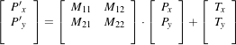 | (3.1) |
Based on the above discussion, we need much smaller scales for translation parameters of vector T (T x, T y) compared to the parameters of matrix M (M11, M12, M21, M22). However, it is not easy to have an intuitive estimation of all parameter scales when we have to deal with a large parameter space.
Fortunately, ITKv4 provides a framework for automated parameter scaling. itk::RegistrationParameterScalesEstimator vastly reduces the difficulty of tuning parameters for different transform/metric combinations. Parameter scales are estimated by analyzing the result of a small parameter update on the change in the magnitude of physical space deformation induced by the transformation.
The impact from a unit change of a parameter may be defined in multiple ways, such as the maximum shift of voxels in index or physical space, or the average norm of transform Jacobian. Filters itk::RegistrationParameterScalesFromPhysicalShift and itk::RegistrationParameterScalesFromIndexShift use the first definition to estimate the scales, while the itk::RegistrationParameterScalesFromJacobian filter estimates scales based on the later definition. In all methods, the goal is to rescale the transform parameters such that a unit change of each scaled parameter will have the same impact on deformation.
In this example the first filter is chosen to estimate the parameter scales. The scales estimator will then be passed to optimizer.
using ScalesEstimatorType =
itk::RegistrationParameterScalesFromPhysicalShift<MetricType>;
ScalesEstimatorType::Pointer scalesEstimator =
ScalesEstimatorType::New();
scalesEstimator->SetMetric( affineMetric );
scalesEstimator->SetTransformForward( true );
affineOptimizer->SetScalesEstimator( scalesEstimator );
The step length has to be proportional to the expected values of the parameters in the search space. Since the expected values of the matrix coefficients are around 1.0, the initial step of the optimization should be a small number compared to 1.0. As a guideline, it is useful to think of the matrix coefficients as combinations of cos(θ) and sin(θ). This leads to use values close to the expected rotation measured in radians. For example, a rotation of 1.0 degree is about 0.017 radians.
However, we need not worry about the above considerations. Thanks to the ScalesEstimator, the initial step size can also be estimated automatically, either at each iteration or only at the first iteration. In this example we choose to estimate learning rate once at the begining of the registration process.
At the second stage, we run two levels of registration, where the second level is run in full resolution in which we do the final adjustments of the output parameters.
constexpr unsigned int numberOfLevels2 = 2;
ARegistrationType::ShrinkFactorsArrayType shrinkFactorsPerLevel2;
shrinkFactorsPerLevel2.SetSize( numberOfLevels2 );
shrinkFactorsPerLevel2[0] = 2;
shrinkFactorsPerLevel2[1] = 1;
ARegistrationType::SmoothingSigmasArrayType smoothingSigmasPerLevel2;
smoothingSigmasPerLevel2.SetSize( numberOfLevels2 );
smoothingSigmasPerLevel2[0] = 1;
smoothingSigmasPerLevel2[1] = 0;
affineRegistration->SetNumberOfLevels ( numberOfLevels2 );
affineRegistration->SetShrinkFactorsPerLevel( shrinkFactorsPerLevel2 );
affineRegistration->SetSmoothingSigmasPerLevel( smoothingSigmasPerLevel2 );
Finally we trigger the registration process by calling Update() and add the output transform of the last stage to the composite transform. This composite transform will be considered as the final transform of this multistage registration process and will be used by the resampler to resample the moving image in to the virtual domain space (fixed image space if there is no fixed initial transform).
try
{
affineRegistration->Update();
std::cout << "Optimizer stop condition: "
<< affineRegistration->GetOptimizer()->GetStopConditionDescription()
<< std::endl;
}
catch( itk::ExceptionObject & err )
{
std::cout << "ExceptionObject caught !" << std::endl;
std::cout << err << std::endl;
return EXIT_FAILURE;
}
compositeTransform->AddTransform(
affineRegistration->GetModifiableTransform() );
Let’s execute this example using the following multi-modality images:
The second image is the result of intentionally rotating the first image by 10 degrees and then translating by (-13,-17). Both images have unit-spacing and are shown in Figure 3.36.
The registration converges after 5 iterations in the translation stage. Also, in the second stage, the registration converges after 46 iterations in the first level, and 6 iterations in the second level. The final results when printed as an array of parameters are:
As it can be seen, the translation parameters after the first stage compensate most of the offset between the fixed and moving images. When the images are close to each other, the affine registration is run for the rotation and the final match. By reordering the Affine array of parameters as coefficients of matrix M and vector T they can now be seen as
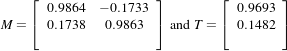 | (3.2) |
In this form, it is easier to interpret the effect of the transform. The matrix M is responsible for scaling, rotation and shearing while T is responsible for translations.
The second component of the matrix values is usually associated with sinθ. We obtain the rotation through SVD of the affine matrix. The value is 9.975 degrees, which is approximately the intentional misalignment of 10.0 degrees.
Also, let’s compute the total translation values resulting from initial transform, translation transform, and the Affine transform together.
In X direction:
 | (3.3) |
In Y direction:
 | (3.4) |
It can be seen that the translation values closely match the true misalignment introduced in the moving image.
It is important to note that once the images are registered at a sub-pixel level, any further improvement of the registration relies heavily on the quality of the interpolator. It may then be reasonable to use a coarse and fast interpolator in the lower resolution levels and switch to a high-quality but slow interpolator in the final resolution level. However, in this example we used a linear interpolator for all stages and different registration levels since it is so fast.


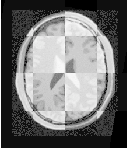
The result of resampling the moving image is presented in the left image of Figure 3.37. The center and right images of the figure depict a checkerboard composite of the fixed and moving images before and after registration.
The source code for this section can be found in the file
MultiStageImageRegistration2.cxx.
This examples shows how different stages can be cascaded together directly in a multistage registration process. The example code is, for the most part, identical to the previous multistage example. The main difference is that no initial transform is used, and the output of the first stage is directly linked to the second stage, and the whole registration process is triggered only once by calling Update() after the last stage stage.
We will focus on the most relevent changes in current code and skip all the similar parts already explained in the previous example.
Let’s start by defining different types of the first stage.
using TTransformType = itk::TranslationTransform< double, Dimension >;
using TOptimizerType = itk::RegularStepGradientDescentOptimizerv4<double>;
using MetricType = itk::MattesMutualInformationImageToImageMetricv4<
FixedImageType,
MovingImageType >;
using TRegistrationType = itk::ImageRegistrationMethodv4<
FixedImageType,
MovingImageType >;
Type definitions are the same as previous example with an important subtle change: the transform type is not passed to the registration method as a template parameter anymore. In this case, the registration filter will consider the transform base class itk::Transform as the type of its output transform.
Instead of passing the transform type, we create an explicit instantiation of the transform object outside of the registration filter, and connect that to the registration object using the SetInitialTransform() method. Also, by calling InPlaceOn() method, this transform object will be the output transform of the registration filter or will be grafted to the output.
Also, there is no initial transform defined for this example.
As in the previous example, the first stage is run using only one level of registration at a coarse resolution level. However, notice that we do not need to update the translation registration filter at this step since the output of this stage will be directly connected to the initial input of the next stage. Due to ITK’s pipeline structure, when we call the Update() at the last stage, the first stage will be updated as well.
Now we upgrade to an Affine transform as the second stage of registration process, and as before, we initially define and instantiate different components of the current registration stage. We have used a new optimizer but the same metric in new configurations.
Again notice that TransformType is not passed to the type definition of the registration filter. It is important because when the registration filter considers transform base class itk::Transform as the type of its output transform, it prevents the type mismatch when the two stages are cascaded to each other.
Then, all components are instantiated using their New() method and connected to the registration object among the transform type. Despite the previous example, here we use the fixed image’s center of mass to initialize the fixed parameters of the Affine transform. itk::ImageMomentsCalculator filter is used for this purpose.
using FixedImageCalculatorType = itk::ImageMomentsCalculator<FixedImageType>;
FixedImageCalculatorType::Pointer fixedCalculator =
FixedImageCalculatorType::New();
fixedCalculator->SetImage( fixedImage );
fixedCalculator->Compute();
FixedImageCalculatorType::VectorType fixedCenter =
fixedCalculator->GetCenterOfGravity();
Then, we initialize the fixed parameters (center of rotation) in the Affine transform and connect that to the registration object.
ATransformType::Pointer affineTx = ATransformType::New();
const unsigned int numberOfFixedParameters =
affineTx->GetFixedParameters().Size();
ATransformType::ParametersType fixedParameters( numberOfFixedParameters );
for (unsigned int i = 0; i < numberOfFixedParameters; ++i)
{
fixedParameters[i] = fixedCenter[i];
}
affineTx->SetFixedParameters( fixedParameters );
affineRegistration->SetInitialTransform( affineTx );
affineRegistration->InPlaceOn();
Now, the output of the first stage is wrapped through a itk::DataObjectDecorator and is passed to the input of the second stage as the moving initial transform via SetMovingInitialTransformInput() method. Note that this API has an “Input” word attached to the name of another initialization method SetMovingInitialTransform() that already has been used in previous example. This extension means that the following API expects a data object decorator type.
Second stage runs two levels of registration, where the second level is run in full resolution.
Once all the registration components are in place, finally we trigger the whole registration process, including two cascaded registration stages, by calling Update() on the registration filter of the last stage, which causes both stages be updated.
try
{
affineRegistration->Update();
std::cout << "Optimizer stop condition: "
<< affineRegistration->
GetOptimizer()->GetStopConditionDescription()
<< std::endl;
}
catch( itk::ExceptionObject & err )
{
std::cout << "ExceptionObject caught !" << std::endl;
std::cout << err << std::endl;
return EXIT_FAILURE;
}
Finally, a composite transform is used to concatenate the results of all stages together, which will be considered as the final output of this multistage process and will be passed to the resampler to resample the moving image into the virtual domain space (fixed image space if there is no fixed initial transform).
Let’s execute this example using the same multi-modality images as before. The registration converges after 6 iterations in the first stage, also in 45 and 11 iterations corresponding to the first level and second level of the Affine stage. The final results when printed as an array of parameters are:
Let’s reorder the Affine array of parameters again as coefficients of matrix M and vector T . They can now be seen as
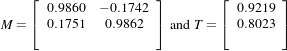 | (3.5) |
10.02 degrees is the rotation value computed from the affine matrix parameters, which approximately equals the intentional misalignment.
Also for the total translation value resulted from both transforms, we have:
In X direction:
 | (3.6) |
In Y direction:
 | (3.7) |
These results closely match the true misalignment introduced in the moving image.


The result of resampling the moving image is presented in the left image of Figure 3.38. The center and right images of the figure depict a checkerboard composite of the fixed and moving images before and after registration.
With the completion of these examples, we will now review the main features of the components forming the registration framework.
In the Insight Toolkit, itk::Transform objects encapsulate the mapping of points and vectors from an input space to an output space. If a transform is invertible, back transform methods are also provided. Currently, ITK provides a variety of transforms from simple translation, rotation and scaling to general affine and kernel transforms. Note that, while in this section we discuss transforms in the context of registration, transforms are general and can be used for other applications. Some of the most commonly used transforms will be discussed in detail later. Let’s begin by introducing the objects used in ITK for representing basic spatial concepts.
ITK implements a consistent geometric representation of space. The characteristics of classes involved in this representation are summarized in Table 3.1. In this regard, ITK takes full advantage of the capabilities of Object Oriented programming and resists the temptation of using simple arrays of float or double in order to represent geometrical objects. The use of basic arrays would have blurred the important distinction between the different geometrical concepts and would have allowed for the innumerable conceptual and programming errors that result from using a vector where a point is needed or vice versa.
| Class | Geometrical concept |
| Position in space. In N-dimensional space it is represented by an array of N numbers associated with space coordinates. |
|
| Relative position between two points. In N-dimensional space it is represented by an array of N numbers, each one associated with the distance along a coordinate axis. Vectors do not have a position in space. A vector is defined as the subtraction of two points. |
|
| Orthogonal direction to a (N - 1)-dimensional manifold in space. For example, in 3D it corresponds to the vector orthogonal to a surface. This is the appropriate class for representing gradients of functions. Covariant vectors do not have a position in space. Covariant vector should not be added to Points, nor to Vectors. |
|
Additional uses of the itk::Point, itk::Vector and itk::CovariantVector classes have been discussed in the Data Representation chaper of Book 1. Each one of these classes behaves differently under spatial transformations. It is therefore quite important to keep their distinction clear. Figure 3.39 illustrates the differences between these concepts.
Transform classes provide different methods for mapping each one of the basic space-representation objects. Points, vectors and covariant vectors are transformed using the methods TransformPoint(), TransformVector() and TransformCovariantVector() respectively.
One of the classes that deserves further comments is the itk::Vector. This ITK class tends to be misinterpreted as a container of elements instead of a geometrical object. This is a common misconception originating from the colloquial use by computer scientists and software engineers of the term “Vector”. The actual word “Vector” is relatively young. It was coined by William Hamilton in his book “Elements of Quaternions” published in 1886 (post-mortem)[24]. In the same text Hamilton coined the terms: “Scalar”, “Versor” and “Tensor”. Although the modern term of “Tensor” is used in Calculus in a different sense of what Hamilton defined in his book at the time [17].
A “Vector” is, by definition, a mathematical object that embodies the concept of “direction in space”. Strictly speaking, a Vector describes the relationship between two Points in space, and captures both their relative distance and orientation.
Computer scientists and software engineers misused the term vector in order to represent the concept of an “Indexed Set” [5]. Mechanical Engineers and Civil Engineers, who deal with the real world of physical objects will not commit this mistake and will keep the word “Vector” attached to a geometrical concept. Biologists, on the other hand, will associate “Vector” to a “vehicle” that allows them to direct something in a particular direction, for example, a virus that allows them to insert pieces of code into a DNA strand [35].
Textbooks in programming do not help to clarify those concepts and loosely use the term “Vector” for the purpose of representing an “enumerated set of common elements”. STL follows this trend and continues using the word “Vector” in this manner [5, 1]. Linear algebra separates the “Vector” from its notion of geometric reality and makes it an abstract set of numbers with arithmetic operations associated.
For those of you who are looking for the “Vector” in the Software Engineering sense, please look at the itk::Array and itk::FixedArray classes that actually provide such functionalities. Additionally, the itk::VectorContainer and itk::MapContainer classes may be of interest too. These container classes are intended for algorithms which require insertion and deletion of elements, and those which may have large numbers of elements.
The Insight Toolkit deals with real objects that inhabit the physical space. This is particularly true in the context of the image registration framework. We chose to give the appropriate name to the mathematical objects that describe geometrical relationships in N-Dimensional space. It is for this reason that we explicitly make clear the distinction between Point, Vector and CovariantVector, despite the fact that most people would be happy with a simple use of double[3] for the three concepts and then will proceed to perform all sort of conceptually flawed operations such as
In order to enforce the correct use of the geometrical concepts in ITK we organized these classes in a hierarchy that supports reuse of code and compartmentalizes the behavior of the individual classes. The use of the itk::FixedArray as the base class of the itk::Point, the itk::Vector and the itk::CovariantVector was a design decision based on the decision to use the correct nomenclature.
An itk::FixedArray is an enumerated collection with a fixed number of elements. You can instantiate a fixed array of letters, or a fixed array of images, or a fixed array of transforms, or a fixed array of geometrical shapes. Therefore, the FixedArray only implements the functionality that is necessary to access those enumerated elements. No assumptions can be made at this point on any other operations required by the elements of the FixedArray, except that it will have a default constructor.
The itk::Point is a type that represents the spatial coordinates of a spatial location. Based on geometrical concepts we defined the valid operations of the Point class. In particular we made sure that no operator+() was defined between Points, and that no operator⋆( scalar ) nor operator/( scalar ) were defined for Points.
In other words, you can perform ITK operations such as:
and you cannot (because you should not) perform operations such as
The itk::Vector is, by Hamilton’s definition, the subtraction between two points. Therefore a Vector must satisfy the following basic operations:
An itk::Vector object is intended to be instantiated over elements that support mathematical operation such as addition, subtraction and multiplication by scalars.
Each transform class typically has several methods for setting its parameters. For example, itk::Euler2DTransform provides methods for specifying the offset, angle, and the entire rotation matrix. However, for use in the registration framework, the parameters are represented by a flat Array of doubles to facilitate communication with generic optimizers. In the case of the Euler2DTransform, the transform is also defined by three doubles: the first representing the angle, and the last two the offset. The flat array of parameters is defined using SetParameters(). A description of the parameters and their ordering is documented in the sections that follow.
In the context of registration, the transform parameters define the search space for optimizers. That is, the goal of the optimization is to find the set of parameters defining a transform that results in the best possible value of an image metric. The more parameters a transform has, the longer its computational time will be when used in a registration method since the dimension of the search space will be equal to the number of transform parameters.
Another requirement that the registration framework imposes on the transform classes is the computation of their Jacobians. In general, metrics require the knowledge of the Jacobian in order to compute Metric derivatives. The Jacobian is a matrix whose elements are the partial derivatives of the output point with respect to the array of parameters that defines the transform:7
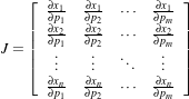 | (3.8) |
where {pi} are the transform parameters and {xi} are the coordinates of the output point. Within this framework, the Jacobian is represented by an itk::Array2D of doubles and is obtained from the transform by method GetJacobian(). The Jacobian can be interpreted as a matrix that indicates for a point in the input space how much its mapping on the output space will change as a response to a small variation in one of the transform parameters. Note that the values of the Jacobian matrix depend on the point in the input space. So actually the Jacobian can be noted as J(X), where X = {xi}. The use of transform Jacobians enables the efficient computation of metric derivatives. When Jacobians are not available, metrics derivatives have to be computed using finite differences at a price of 2M evaluations of the metric value, where M is the number of transform parameters.
The following sections describe the main characteristics of the transform classes available in ITK.
| Behavior | Number of Parameters | Parameter Ordering | Restrictions |
| Maps every point to itself, every vector to itself and every covariant vector to itself. | 0 | NA | Only defined when the input and output space has the same number of dimensions. |
The identity transform itk::IdentityTransform is mainly used for debugging purposes. It is provided to methods that require a transform and in cases where we want to have the certainty that the transform will have no effect whatsoever in the outcome of the process. The main characteristics of the identity transform are summarized in Table 3.2
| Behavior | Number of Parameters | Parameter Ordering | Restrictions |
| Represents a simple translation of points in the input space and has no effect on vectors or covariant vectors. | Same as the input space dimension. | The i-th parameter represents the translation in the i-th dimension. | Only defined when the input and output space have the same number of dimensions. |
The itk::TranslationTransform is probably the simplest yet one of the most useful transformations. It maps all Points by adding a Vector to them. Vector and covariant vectors remain unchanged under this transformation since they are not associated with a particular position in space. Translation is the best transform to use when starting a registration method. Before attempting to solve for rotations or scaling it is important to overlap the anatomical objects in both images as much as possible. This is done by resolving the translational misalignment between the images. Translations also have the advantage of being fast to compute and having parameters that are easy to interpret. The main characteristics of the translation transform are presented in Table 3.3.
| Behavior | Number of Parameters | Parameter Ordering | Restrictions |
| Points are transformed by multiplying each one of their coordinates by the corresponding scale factor for the dimension. Vectors are transformed as points. Covariant vectors are transformed by dividing their components by the scale factor in the corresponding dimension. | Same as the input space dimension. | The i-th parameter represents the scaling in the i-th dimension. | Only defined when the input and output space have the same number of dimensions. |
The itk::ScaleTransform represents a simple scaling of the vector space. Different scaling factors can be applied along each dimension. Points are transformed by multiplying each one of their coordinates by the corresponding scale factor for the dimension. Vectors are transformed in the same way as points. Covariant vectors, on the other hand, are transformed differently since anisotropic scaling does not preserve angles. Covariant vectors are transformed by dividing their components by the scale factor of the corresponding dimension. In this way, if a covariant vector was orthogonal to a vector, this orthogonality will be preserved after the transformation. The following equations summarize the effect of the transform on the basic geometric objects.
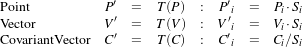 | (3.9) |
where Pi, Vi and Ci are the point, vector and covariant vector i-th components while Si is the scaling factor along dimension i-th. The following equation illustrates the effect of the scaling transform on a 3D point.
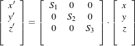 | (3.10) |
Scaling appears to be a simple transformation but there are actually a number of issues to keep in mind when using different scale factors along every dimension. There are subtle effects—for example, when computing image derivatives. Since derivatives are represented by covariant vectors, their values are not intuitively modified by scaling transforms.
One of the difficulties with managing scaling transforms in a registration process is that typical optimizers manage the parameter space as a vector space where addition is the basic operation. Scaling is better treated in the frame of a logarithmic space where additions result in regular multiplicative increments of the scale. Gradient descent optimizers have trouble updating step length, since the effect of an additive increment on a scale factor diminishes as the factor grows. In other words, a scale factor variation of (1.0+ϵ) is quite different from a scale variation of (5.0+ϵ).
Registrations involving scale transforms require careful monitoring of the optimizer parameters in order to keep it progressing at a stable pace. Note that some of the transforms discussed in following sections, for example, the AffineTransform, have hidden scaling parameters and are therefore subject to the same vulnerabilities of the ScaleTransform.
In cases involving misalignments with simultaneous translation, rotation and scaling components it may be desirable to solve for these components independently. The main characteristics of the scale transform are presented in Table 3.4.
| Behavior | Number of Parameters | Parameter Ordering | Restrictions |
| Points are transformed by multiplying each one of their coordinates by the corresponding scale factor for the dimension. Vectors are transformed as points. Covariant vectors are transformed by dividing their components by the scale factor in the corresponding dimension. | Same as the input space dimension. | The i-th parameter represents the scaling in the i-th dimension. | Only defined when the input and output space have the same number of dimensions. The difference between this transform and the ScaleTransform is that here the scaling factors are passed as logarithms, in this way their behavior is closer to the one of a Vector space. |
The itk::ScaleLogarithmicTransform is a simple variation of the itk::ScaleTransform. It is intended to improve the behavior of the scaling parameters when they are modified by optimizers. The difference between this transform and the ScaleTransform is that the parameter factors are passed here as logarithms. In this way, multiplicative variations in the scale become additive variations in the logarithm of the scaling factors.
| Behavior | Number of Parameters | Parameter Ordering | Restrictions |
| Represents a 2D rotation and a 2D translation. Note that the translation component has no effect on the transformation of vectors and covariant vectors. | 3 | The first parameter is the angle in radians and the last two parameters are the translation in each dimension. | Only defined for two-dimensional input and output spaces. |
itk::Euler2DTransform implements a rigid transformation in 2D. It is composed of a plane rotation and a two-dimensional translation. The rotation is applied first, followed by the translation. The following equation illustrates the effect of this transform on a 2D point,
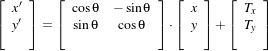 | (3.11) |
where θ is the rotation angle and (T x,T y) are the components of the translation.
A challenging aspect of this transformation is the fact that translations and rotations do not form a vector space and cannot be managed as linearly independent parameters. Typical optimizers make the loose assumption that parameters exist in a vector space and rely on the step length to be small enough for this assumption to hold approximately.
In addition to the non-linearity of the parameter space, the most common difficulty found when using this transform is the difference in units used for rotations and translations. Rotations are measured in radians; hence, their values are in the range [-π,π]. Translations are measured in millimeters and their actual values vary depending on the image modality being considered. In practice, translations have values on the order of 10 to 100. This scale difference between the rotation and translation parameters is undesirable for gradient descent optimizers because they deviate from the trajectories of descent and make optimization slower and more unstable. In order to compensate for these differences, ITK optimizers accept an array of scale values that are used to normalize the parameter space.
Registrations involving angles and translations should take advantage of the scale normalization functionality in order to obtain the best performance out of the optimizers. The main characteristics of the Euler2DTransform class are presented in Table 3.6.
| Behavior | Number of Parameters | Parameter Ordering | Restrictions |
| Represents a 2D rotation around a user-provided center followed by a 2D translation. | 5 | The first parameter is the angle in radians. Second and third are the center of rotation coordinates and the last two parameters are the translation in each dimension. | Only defined for two-dimensional input and output spaces. |
itk::CenteredRigid2DTransform implements a rigid transformation in 2D. The main difference between this transform and the itk::Euler2DTransform is that here we can specify an arbitrary center of rotation, while the Euler2DTransform always uses the origin of the coordinate system as the center of rotation. This distinction is quite important in image registration since ITK images usually have their origin in the corner of the image rather than the middle. Rotational mis-registrations usually exist, however, as rotations around the center of the image, or at least as rotations around a point in the middle of the anatomical structure captured by the image. Using gradient descent optimizers, it is almost impossible to solve non-origin rotations using a transform with origin rotations since the deep basin of the real solution is usually located across a high ridge in the topography of the cost function.
In practice, the user must supply the center of rotation in the input space, the angle of rotation and a translation to be applied after the rotation. With these parameters, the transform initializes a rotation matrix and a translation vector that together perform the equivalent of translating the center of rotation to the origin of coordinates, rotating by the specified angle, translating back to the center of rotation and finally translating by the user-specified vector.
As with the Euler2DTransform, this transform suffers from the difference in units used for rotations and translations. Rotations are measured in radians; hence, their values are in the range [-π,π]. The center of rotation and the translations are measured in millimeters, and their actual values vary depending on the image modality being considered. Registrations involving angles and translations should take advantage of the scale normalization functionality of the optimizers in order to get the best performance out of them.
The following equation illustrates the effect of the transform on an input point (x,y) that maps to the output point (x′,y′),
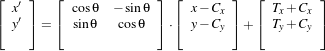 | (3.12) |
where θ is the rotation angle, (Cx,Cy) are the coordinates of the rotation center and (T x,T y) are the components of the translation. Note that the center coordinates are subtracted before the rotation and added back after the rotation. The main features of the CenteredRigid2DTransform are presented in Table 3.7.
| Behavior | Number of Parameters | Parameter Ordering | Restrictions |
| Represents a 2D rotation, homogeneous scaling and a 2D translation. Note that the translation component has no effect on the transformation of vectors and covariant vectors. | 4 | The first parameter is the scaling factor for all dimensions, the second is the angle in radians, and the last two parameters are the translations in (x,y) respectively. | Only defined for two-dimensional input and output spaces. |
The itk::Similarity2DTransform can be seen as a rigid transform combined with an isotropic scaling factor. This transform preserves angles between lines. In its 2D implementation, the four parameters of this transformation combine the characteristics of the itk::ScaleTransform and itk::Euler2DTransform. In particular, those relating to the non-linearity of the parameter space and the non-uniformity of the measurement units. Gradient descent optimizers should be used with caution on such parameter spaces since the notions of gradient direction and step length are ill-defined.
The following equation illustrates the effect of the transform on an input point (x,y) that maps to the output point (x′,y′),
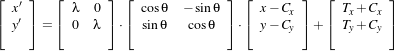 | (3.13) |
where λ is the scale factor, θ is the rotation angle, (Cx,Cy) are the coordinates of the rotation center and (T x,T y) are the components of the translation. Note that the center coordinates are subtracted before the rotation and scaling, and they are added back afterwards. The main features of the Similarity2DTransform are presented in Table 3.8.
A possible approach for controlling optimization in the parameter space of this transform is to dynamically modify the array of scales passed to the optimizer. The effect produced by the parameter scaling can be used to steer the walk in the parameter space (by giving preference to some of the parameters over others). For example, perform some iterations updating only the rotation angle, then balance the array of scale factors in the optimizer and perform another set of iterations updating only the translations.
| Behavior | Number of Parameters | Parameter Ordering | Restrictions |
| Represents a 3D rotation and a 3D translation. The rotation is specified as a quaternion, defined by a set of four numbers q. The relationship between quaternion and rotation about vector n by angle θ is as follows:  Note that if the quaternion is not of unit length, scaling will also result. | 7 | The first four parameters defines the quaternion and the last three parameters the translation in each dimension. | Only defined for three-dimensional input and output spaces. |
The itk::QuaternionRigidTransform class implements a rigid transformation in 3D space. The rotational part of the transform is represented using a quaternion while the translation is represented with a vector. Quaternions components do not form a vector space and hence raise the same concerns as the itk::Similarity2DTransform when used with gradient descent optimizers.
The itk::QuaternionRigidTransformGradientDescentOptimizer was introduced into the toolkit to address these concerns. This specialized optimizer implements a variation of a gradient descent algorithm adapted for a quaternion space. This class ensures that after advancing in any direction on the parameter space, the resulting set of transform parameters is mapped back into the permissible set of parameters. In practice, this comes down to normalizing the newly-computed quaternion to make sure that the transformation remains rigid and no scaling is applied. The main characteristics of the QuaternionRigidTransform are presented in Table 3.9.
The Quaternion rigid transform also accepts a user-defined center of rotation. In this way, the transform can easily be used for registering images where the rotation is mostly relative to the center of the image instead of one of the corners. The coordinates of this rotation center are not subject to optimization. They only participate in the computation of the mappings for Points and in the computation of the Jacobian. The transformations for Vectors and CovariantVector are not affected by the selection of the rotation center.
| Behavior | Number of Parameters | Parameter Ordering | Restrictions |
| Represents a 3D rotation. The rotation is specified by a versor or unit quaternion. The rotation is performed around a user-specified center of rotation. | 3 | The three parameters define the versor. | Only defined for three-dimensional input and output spaces. |
By definition, a Versor is the rotational part of a Quaternion. It can also be defined as a unit-quaternion [24, 27]. Versors only have three independent components, since they are restricted to reside in the space of unit-quaternions. The implementation of versors in the toolkit uses a set of three numbers. These three numbers correspond to the first three components of a quaternion. The fourth component of the quaternion is computed internally such that the quaternion is of unit length. The main characteristics of the itk::VersorTransform are presented in Table 3.10.
This transform exclusively represents rotations in 3D. It is intended to rapidly solve the rotational component of a more general misalignment. The efficiency of this transform comes from using a parameter space of reduced dimensionality. Versors are the best possible representation for rotations in 3D space. Sequences of versors allow the creation of smooth rotational trajectories; for this reason, they behave stably under optimization methods.
The space formed by versor parameters is not a vector space. Standard gradient descent algorithms are not appropriate for exploring this parameter space. An optimizer specialized for the versor space is available in the toolkit under the name of itk::VersorTransformOptimizer. This optimizer implements versor derivatives as originally defined by Hamilton [24].
The center of rotation can be specified by the user with the SetCenter() method. The center is not part of the parameters to be optimized, therefore it remains the same during an optimization process. Its value is used during the computations for transforming Points and when computing the Jacobian.
| Behavior | Number of Parameters | Parameter Ordering | Restrictions |
| Represents a 3D rotation and a 3D translation. The rotation is specified by a versor or unit quaternion, while the translation is represented by a vector. Users can specify the coordinates of the center of rotation. | 6 | The first three parameters define the versor and the last three parameters the translation in each dimension. | Only defined for three-dimensional input and output spaces. |
The itk::VersorRigid3DTransform implements a rigid transformation in 3D space. It is a variant of the itk::QuaternionRigidTransform and the itk::VersorTransform. It can be seen as a itk::VersorTransform plus a translation defined by a vector. The advantage of this class with respect to the QuaternionRigidTransform is that it exposes only six parameters, three for the versor components and three for the translational components. This reduces the search space for the optimizer to six dimensions instead of the seven dimensional used by the QuaternionRigidTransform. This transform also allows the users to set a specific center of rotation. The center coordinates are not modified during the optimization performed in a registration process. The main features of this transform are summarized in Table 3.11. This transform is probably the best option to use when dealing with rigid transformations in 3D.
Given that the space of Versors is not a Vector space, typical gradient descent optimizers are not well suited for exploring the parametric space of this transform. The itk::VersorRigid3DTranformOptimizer has been introduced in the ITK toolkit with the purpose of providing an optimizer that is aware of the Versor space properties on the rotational part of this transform, as well as the Vector space properties on the translational part of the transform.
| Behavior | Number of Parameters | Parameter Ordering | Restrictions |
| Represents a rigid rotation in 3D space. That is, a rotation followed by a 3D translation. The rotation is specified by three angles representing rotations to be applied around the X, Y and Z axes one after another. The translation part is represented by a Vector. Users can also specify the coordinates of the center of rotation. | 6 | The first three parameters are the rotation angles around X, Y and Z axes, and the last three parameters are the translations along each dimension. | Only defined for three-dimensional input and output spaces. |
The itk::Euler3DTransform implements a rigid transformation in 3D space. It can be seen as a rotation followed by a translation. This class exposes six parameters, three for the Euler angles that represent the rotation and three for the translational components. This transform also allows the users to set a specific center of rotation. The center coordinates are not modified during the optimization performed in a registration process. The main features of this transform are summarized in Table 3.12.
Three rotational parameters are non-linear and do not behave like Vector spaces. This must be taken into account when selecting an optimizer to work with this transform and when fine tuning the parameters of the optimizer. It is strongly recommended to use this transform by introducing very small variations on the rotational components. A small rotation will be in the range of 1 degree, which in radians is approximately 0.01745.
You should not expect this transform to be able to compensate for large rotations just by being driven with the optimizer. In practice you must provide a reasonable initialization of the transform angles and only need to correct for residual rotations in the order of 10 or 20 degrees.
| Behavior | Number of Parameters | Parameter Ordering | Restrictions |
| Represents a 3D rotation, a 3D translation and homogeneous scaling. The scaling factor is specified by a scalar, the rotation is specified by a versor, and the translation is represented by a vector. Users can also specify the coordinates of the center of rotation, which is the same center used for scaling. | 7 | The first three parameters define the Versor, the next three parameters the translation in each dimension, and the last parameter is the isotropic scaling factor. | Only defined for three-dimensional input and output spaces. |
The itk::Similarity3DTransform implements a similarity transformation in 3D space. It can be seen as an homogeneous scaling followed by a itk::VersorRigid3DTransform. This class exposes seven parameters: one for the scaling factor, three for the versor components and three for the translational components. This transform also allows the user to set a specific center of rotation. The center coordinates are not modified during the optimization performed in a registration process. Both the rotation and scaling operations are performed with respect to the center of rotation. The main features of this transform are summarized in Table 3.13.
The scaling and rotational spaces are non-linear and do not behave like Vector spaces. This must be taken into account when selecting an optimizer to work with this transform and when fine tuning the parameters of the optimizer.
| Behavior | Number of Parameters | Parameter Ordering | Restrictions |
| Represents a rigid 3D transformation followed by a perspective projection. The rotation is specified by a Versor, while the translation is represented by a Vector. Users can specify the coordinates of the center of rotation. They must specify a focal distance to be used for the perspective projection. The rotation center and the focal distance parameters are not modified during the optimization process. | 6 | The first three parameters define the Versor and the last three parameters the Translation in each dimension. | Only defined for three-dimensional input and two-dimensional output spaces. This is one of the few transforms where the input space has a different dimension from the output space. |
The itk::Rigid3DPerspectiveTransform implements a rigid transformation in 3D space followed by a perspective projection. This transform is intended to be used in 3D∕2D registration problems where a 3D object is projected onto a 2D plane. This is the case in Fluoroscopic images used for image-guided intervention, and it is also the case for classical radiography. Users must provide a value for the focal distance to be used during the computation of the perspective transform. This transform also allows users to set a specific center of rotation. The center coordinates are not modified during the optimization performed in a registration process. The main features of this transform are summarized in Table 3.14. This transform is also used when creating Digitally Reconstructed Radiographs (DRRs).
The strategies for optimizing the parameters of this transform are the same ones used for optimizing the VersorRigid3DTransform. In particular, you can use the same VersorRigid3DTranformOptimizer in order to optimize the parameters of this class.
| Behavior | Number of Parameters | Parameter Ordering | Restrictions |
| Represents an affine transform composed of rotation, scaling, shearing and translation. The transform is specified by a N × N matrix and a N × 1 vector where N is the space dimension. | (N +1)×N | The first N ×N parameters define the matrix in column-major order (where the column index varies the fastest). The last N parameters define the translations for each dimension. | Only defined when the input and output space have the same dimension. |
The itk::AffineTransform is one of the most popular transformations used for image registration. Its main advantage comes from its representation as a linear transformation. The main features of this transform are presented in Table 3.15.
The set of AffineTransform coefficients can actually be represented in a vector space of dimension (N +1)×N. This makes it possible for optimizers to be used appropriately on this search space. However, the high dimensionality of the search space also implies a high computational complexity of cost-function derivatives. The best compromise in the reduction of this computational time is to use the transform’s Jacobian in combination with the image gradient for computing the cost-function derivatives.
The coefficients of the N ×N matrix can represent rotations, anisotropic scaling and shearing. These coefficients are usually of a very different dynamic range compared to the translation coefficients. Coefficients in the matrix tend to be in the range [-1 : 1], but are not restricted to this interval. Translation coefficients, on the other hand, can be on the order of 10 to 100, and are basically related to the image size and pixel spacing.
This difference in scale makes it necessary to take advantage of the functionality offered by the optimizers for rescaling the parameter space. This is particularly relevant for optimizers based on gradient descent approaches. This transform lets the user set an arbitrary center of rotation. The coordinates of the rotation center do not make part of the parameters array passed to the optimizer. Equation 3.14 illustrates the effect of applying the AffineTransform to a point in 3D space.
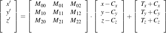 | (3.14) |
A registration based on the affine transform may be more effective when applied after simpler transformations have been used to remove the major components of misalignment. Otherwise it will incur an overwhelming computational cost. For example, using an affine transform, the first set of optimization iterations would typically focus on removing large translations. This task could instead be accomplished by a translation transform in a parameter space of size N instead of the (N +1)×N associated with the affine transform.
Tracking the evolution of a registration process that uses AffineTransforms can be challenging, since it is difficult to represent the coefficients in a meaningful way. A simple printout of the transform coefficients generally does not offer a clear picture of the current behavior and trend of the optimization. A better implementation uses the affine transform to deform a wire-frame cube which is shown in a 3D visualization display.
| Behavior | Number of Parameters | Parameter Ordering | Restrictions |
| Represents a free-form deformation by providing a deformation field from the interpolation of deformations in a coarse grid. | M×N | Where M is the number of nodes in the BSpline grid and N is the dimension of the space. | Only defined when the input and output space have the same dimension. This transform has the advantage of being able to compute deformable registration. It also has the disadvantage of a very high-dimensional parametric space, and therefore requiring long computation times. |
The itk::BSplineDeformableTransform is designed to be used for solving deformable registration problems. This transform is equivalent to generating a deformation field where a deformation vector is assigned to every point in space. The deformation vectors are computed using BSpline interpolation from the deformation values of points located in a coarse grid, which is usually referred to as the BSpline grid.
The BSplineDeformableTransform is not flexible enough to account for large rotations or shearing, or scaling differences. In order to compensate for this limitation, it provides the functionality of being composed with an arbitrary transform. This transform is known as the Bulk transform and it applied to points before they are mapped with the displacement field.
This transform does not provide functionality for mapping Vectors nor CovariantVectors—only Points can be mapped. This is because the variations of a vector under a deformable transform actually depend on the location of the vector in space. In other words, Vectors only make sense as the relative position between two points.
The BSplineDeformableTransform has a very large number of parameters and therefore is well suited for the itk::LBFGSOptimizer and itk::LBFGSBOptimizer. The use of this transform was proposed in the following papers [52, 39, 40].
Kernel Transforms are a set of Transforms that are also suitable for performing deformable registration. These transforms compute on-the-fly the displacements corresponding to a deformation field. The displacement values corresponding to every point in space are computed by interpolation from the vectors defined by a set of Source Landmarks and a set of Target Landmarks.
Several variations of these transforms are available in the toolkit. They differ in the type of interpolation kernel that is used when computing the deformation in a particular point of space. Note that these transforms are computationally expensive and that their numerical complexity is proportional to the number of landmarks and the space dimension.
The following is the list of Transforms based on the KernelTransform.
Details about the mathematical background of these transform can be found in the paper by Davis et. al [14] and the papers by Rohr et. al [50, 51].
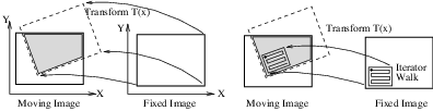
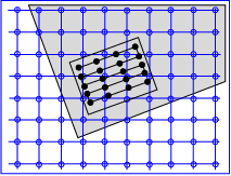
Figure 3.41: Grid positions of the fixed image
map to non-grid positions of the moving image.
In the registration process, the metric typically compares intensity values in the fixed image against the corresponding values in the transformed moving image. When a point is mapped from one space to another by a transform, it will in general be mapped to a non-grid position. Therefore, interpolation is required to evaluate the image intensity at the mapped position.
Figure 3.40 (left) illustrates the mapping of the fixed image space onto the moving image space. The transform maps points from the fixed image coordinate system onto the moving image coordinate system. The figure highlights the region of overlap between the two images after the mapping. The right side illustrates how an iterator is used to walk through a region of the fixed image. Each one of the iterator positions is mapped by the transform onto the moving image space in order to find the homologous pixel.
Figure 3.41 presents a detailed view of the mapping from the fixed image to the moving image. In general, the grid positions of the fixed image will not be mapped onto grid positions of the moving image. Interpolation is needed for estimating the intensity of the moving image at these non-grid positions. The service is provided in ITK by interpolator classes that can be plugged into the registration method.
The following interpolators are available:
In the context of registration, the interpolation method affects the smoothness of the optimization search space and the overall computation time. On the other hand, interpolations are executed thousands of times in a single optimization cycle. Hence, the user has to balance the simplicity of computation with the smoothness of the optimization when selecting the interpolation scheme.
The basic input to an itk::InterpolateImageFunction is the image to be interpolated. Once an image has been defined using SetInputImage(), a user can interpolate either at a point using Evaluate() or an index using EvaluateAtContinuousIndex().
Interpolators provide the method IsInsideBuffer() that tests whether a particular image index or a physical point falls inside the spatial domain for which image pixels exist.
The itk::NearestNeighborInterpolateImageFunction simply uses the intensity of the nearest grid position. That is, it assumes that the image intensity is piecewise constant with jumps mid-way between grid positions. This interpolation scheme is cheap as it does not require any floating point computations.
The itk::LinearInterpolateImageFunction assumes that intensity varies linearly between grid positions. Unlike nearest neighbor interpolation, the interpolated intensity is spatially continuous. However, the intensity gradient will be discontinuous at grid positions.
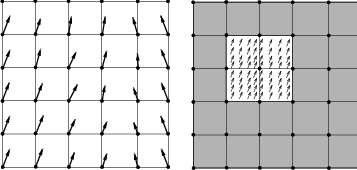
The itk::BSplineInterpolateImageFunction represents the image intensity using B-spline basis functions. When an input image is first connected to the interpolator, B-spline coefficients are computed using recursive filtering (assuming mirror boundary conditions). Intensity at a non-grid position is computed by multiplying the B-spline coefficients with shifted B-spline kernels within a small support region of the requested position. Figure 3.42 illustrates on the left how the deformation values on the BSpline grid nodes are used for computing interpolated deformations in the rest of space. Note for example that when a cubic BSpline is used, the grid must have one extra node in one side of the image and two extra nodes on the other side, this along every dimension.
Currently, this interpolator supports splines of order 0 to 5. Using a spline of order 0 is almost identical to nearest neighbor interpolation; a spline of order 1 is exactly identical to linear interpolation. For splines of order greater than 1, both the interpolated value and its derivative are spatially continuous.
It is important to note that when using this scheme, the interpolated value may lie outside the range of input image intensities. This is especially important when handling unsigned data, as it is possible that the interpolated value is negative.
The itk::WindowedSincInterpolateImageFunction is the best possible interpolator for data that have been digitized in a discrete grid. This interpolator has been developed based on Fourier Analysis considerations. It is well known in signal processing that the process of sampling a spatial function using a periodic discrete grid results in a replication of the spectrum of that signal in the frequency domain.
The process of recovering the continuous signal from the discrete sampling is equivalent to the removal of the replicated spectra in the frequency domain. This can be done by multiplying the spectra with a box function that will set to zero all the frequencies above the highest frequency in the original signal. Multiplying the spectrum with a box function is equivalent to convolving the spatial discrete signal with a sinc function
 | (3.15) |
The sinc function has infinite support, which of course in practice can not really be implemented. Therefore, the sinc is usually truncated by multiplying it with a Window function. The Windowed Sinc interpolator is the result of such an operation.
This interpolator presents a series of trade-offs in its utilization. Probably the most significant is that the larger the window, the more precise will be the resulting interpolation. However, large windows will also result in long computation times. Since the user can select the window size in this interpolator, it is up to the user to determine how much interpolation quality is required in her/his application and how much computation time can be justified. For details on the signal processing theory behind this interpolator, please refer to Meijering et. al [41].
The region of the image used for computing the interpolator is determined by the window radius. For example, in a 2D image where we want to interpolate the value at position (x,y) the following computation will be performed.
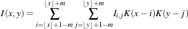 | (3.16) |
where m is the radius of the window. Typically, values such as 3 or 4 are reasonable for the window radius. The function kernel K(t) is composed by the sinc function and one of the windows listed above.
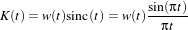 | (3.17) |
Some of the windows that can be used with this interpolator are
Cosinus window
 | (3.18) |
Hamming window
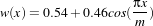 | (3.19) |
Welch window
 | (3.20) |
Lancos window
 | (3.21) |
Blackman window
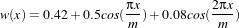 | (3.22) |
The window functions listed above are available inside the itk::Function namespace. The conclusions of the referenced paper suggest to use the Welch, Cosine, Kaiser, and Lancos windows for m = 4,5. These are based on error in rotating medical images with respect to the linear interpolation method. In some cases the results achieve a 20-fold improvement in accuracy.
This filter can be used in the same way you would use any ImageInterpolationFunction. For instance, you can plug it into the ResampleImageFilter class. In order to instantiate the filter you must choose several template parameters.
TInputImage is the image type, as for any other interpolator.
VRadius is the radius of the kernel, i.e., the m from the formula above.
TWindowFunction is the window function object, which you can choose from about five different functions defined in this header. The default is the Hamming window, which is commonly used but not optimal according to the cited paper.
TBoundaryCondition is the boundary condition class used to determine the values of pixels that fall off the image boundary. This class has the same meaning here as in the itk::NeighborhoodIterator classes.
TCoordRep is again standard for interpolating functions, and should be float or double.
The WindowedSincInterpolateImageFunction is probably not the interpolator that you want to use for performing registration. Its computation burden makes it too expensive for this purpose. The best use of this interpolator is for the final resampling of the image, once the transform has been found using another less expensive interpolator in the registration process.
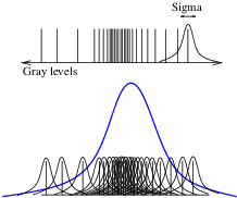
Figure 3.43: In Parzen windowing, a continuous
density function is constructed by superimposing
kernel functions (Gaussian function in this case)
centered on the intensity samples obtained from
the image.
In ITK, itk::ImageToImageMetricv4 objects quantitatively measure how well the transformed moving image fits the fixed image by comparing the gray-scale intensity of the images. These metrics are very flexible and can work with any transform or interpolation method and do not require reduction of the gray-scale images to sparse extracted information such as edges.
The metric component is perhaps the most critical element of the registration framework. The selection of which metric to use is highly dependent on the registration problem to be solved. For example, some metrics have a large capture range while others require initialization close to the optimal position. In addition, some metrics are only suitable for comparing images obtained from the same imaging modality, while others can handle inter-modality comparisons. Unfortunately, there are no clear-cut rules as to how to choose a metric.
The matching Metric class controls most parts of the registration process since it handles fixed, moving and virtual images as well as fixed and moving transforms and interpolators. The method GetValue() can be used to evaluate the quantitative criterion at the transform parameters specified in the argument. Typically, the metric samples points within a defined region of the virtual lattice. For each point, the corresponding fixed and moving image positions are computed using the fixed initial transform and the moving transform with the specified parameters. Then, the fixed and moving interpolators are used to compute the fixed and moving image’s intensities at the mapped positions. Details on this mapping are illustrated in Figures 3.40 and 3.41 assuming that virtual lattice is the same as the fixed image lattice, which is usually the case in practice.
The metrics also support region-based evaluation. The SetFixedImageMask() and SetMovingImageMask() methods may be used to restrict evaluation of the metric within a specified region. The masks may be of any type derived from itk::SpatialObject.
Besides the measure value, gradient-based optimization schemes also require derivatives of the measure with respect to each transform parameter. The methods GetDerivatives() and GetValueAndDerivatives() can be used to obtain the gradient information.
The following is the list of metrics currently available in ITKv4 registration framework:
Also, in case you are interested in using the legacy ITK registration framework, the following is the list of metrics currently available in ITKv3:
In the following sections, we describe the ITKv4 metric types in detail. You can check ITK descriptions in doxygen for details about ITKv3 metric classes.
For ease of notation, we will refer to the fixed image f(X) and transformed moving image (m∘T (X)) as images A and B.
The itk::MeanSquaresImageToImageMetricv4 computes the mean squared pixel-wise difference in intensity between image A and B over a user defined region:
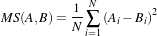 | (3.23) |
Ai is the i-th pixel of Image A
Bi is the i-th pixel of Image B
N is the number of pixels considered
The optimal value of the metric is zero. Poor matches between images A and B result in large values of the metric. This metric is simple to compute and has a relatively large capture radius.
This metric relies on the assumption that intensity representing the same homologous point must be the same in both images. Hence, its use is restricted to images of the same modality. Additionally, any linear changes in the intensity result in a poor match value.
Getting familiar with the characteristics of the Metric as a cost function is fundamental in order to find the best way of setting up an optimization process that will use this metric for solving a registration problem. The following example illustrates a typical mechanism for studying the characteristics of a Metric. Although the example is using the Mean Squares metric, the same methodology can be applied to any of the other metrics available in the toolkit.
The source code for this section can be found in the file
MeanSquaresImageMetric1.cxx.
This example illustrates how to explore the domain of an image metric. This is a useful exercise before starting a registration process, since familiarity with the characteristics of the metric is fundamental for appropriate selection of the optimizer and its parameters used to drive the registration process. This process helps identify how noisy a metric may be in a given range of parameters, and it will also give an idea of the number of local minima or maxima in which an optimizer may get trapped while exploring the parametric space.
We start by including the headers of the basic components: Metric, Transform and Interpolator.
We define the dimension and pixel type of the images to be used in the evaluation of the Metric.
The type of the Metric is instantiated and one is constructed. In this case we decided to use the same image type for both the fixed and the moving images.
We also instantiate the transform and interpolator types, and create objects of each class.
The classes required by the metric are connected to it. This includes the fixed and moving images, the interpolator and the transform.
Note that the SetTransform() method is equivalent to the SetMovingTransform() function. In this example there is no need to use the SetFixedTransform(), since the virtual domain is assumed to be the same as the fixed image domain set as following.
Finally we select a region of the parametric space to explore. In this case we are using a translation transform in 2D, so we simply select translations from a negative position to a positive position, in both x and y. For each one of those positions we invoke the GetValue() method of the Metric.
MetricType::MovingTransformParametersType displacement( Dimension );
constexpr int rangex = 50;
constexpr int rangey = 50;
for( int dx = -rangex; dx <= rangex; dx++ )
{
for( int dy = -rangey; dy <= rangey; dy++ )
{
displacement[0] = dx;
displacement[1] = dy;
metric->SetParameters( displacement );
const double value = metric->GetValue();
std::cout << dx << " " << dy << " " << value << std::endl;
}
}
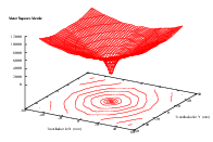
Running this code using the image BrainProtonDensitySlice.png as both the fixed and the moving images results in the plot shown in Figure 3.44. From this figure, it can be seen that a gradient-based optimizer will be appropriate for finding the extrema of the Metric. It is also possible to estimate a good value for the step length of a gradient-descent optimizer.
This exercise of plotting the Metric is probably the best thing to do when a registration process is not converging and when it is unclear how to fine tune the different parameters involved in the registration. This includes the optimizer parameters, the metric parameters and even options such as preprocessing the image data with smoothing filters.
The shell and Gnuplot8 scripts used for generating the graphics in Figure 3.44 are available in the directory
ITKSoftwareGuide/SoftwareGuide/Art
Of course, this plotting exercise becomes more challenging when the transform has more than three parameters, and when those parameters have very different value ranges. In those cases it is necessary to select only a key subset of parameters from the transform and to study the behavior of the metric when those parameters are varied.
The itk::CorrelationImageToImageMetricv4 computes pixel-wise cross-correlation and normalizes it by the square root of the autocorrelation of the images:
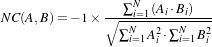 | (3.24) |
Ai is the i-th pixel of Image A
Bi is the i-th pixel of Image B
N is the number of pixels considered
Note the -1 factor in the metric computation. This factor is used to make the metric be optimal when its minimum is reached. The optimal value of the metric is then minus one. Misalignment between the images results in small measure values. The use of this metric is limited to images obtained using the same imaging modality. The metric is insensitive to multiplicative factors between the two images. This metric produces a cost function with sharp peaks and well-defined minima. On the other hand, it has a relatively small capture radius.
The itk::MattesMutualInformationImageToImageMetricv4 computes the mutual information between image A and image B. Mutual information (MI) measures how much information one random variable (image intensity in one image) tells about another random variable (image intensity in the other image). The major advantage of using MI is that the actual form of the dependency does not have to be specified. Therefore, complex mapping between two images can be modeled. This flexibility makes MI well suited as a criterion of multi-modality registration [46].
Mutual information is defined in terms of entropy. Let
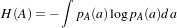 | (3.25) |
be the entropy of random variable A, H(B) the entropy of random variable B and
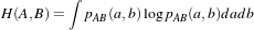 | (3.26) |
be the joint entropy of A and B. If A and B are independent, then
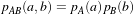 | (3.27) |
and
 | (3.28) |
However, if there is any dependency, then
 | (3.29) |
The difference is called Mutual Information : 
 | (3.30) |
In a typical registration problem, direct access to the marginal and joint probability densities is not available and hence the densities must be estimated from the image data. Parzen windows (also known as kernel density estimators) can be used for this purpose. In this scheme, the densities are constructed by taking intensity samples S from the image and super-positioning kernel functions K(⋅) centered on the elements of S as illustrated in Figure 3.43:
A variety of functions can be used as the smoothing kernel with the requirement that they are smooth, symmetric, have zero mean and integrate to one. For example, boxcar, Gaussian and B-spline functions are suitable candidates. A smoothing parameter is used to scale the kernel function. The larger the smoothing parameter, the wider the kernel function used and hence the smoother the density estimate. If the parameter is too large, features such as modes in the density will get smoothed out. On the other hand, if the smoothing parameter is too small, the resulting density may be too noisy. The estimation is given by the following equation.
 | (3.31) |
Choosing the optimal smoothing parameter is a difficult research problem and beyond the scope of this software guide. Typically, the optimal value of the smoothing parameter will depend on the data and the number of samples used.
The implementation of mutual information metric available in ITKv4 follows the method specified by Mattes et al. in [39] and is implemented by the itk::MattesMutualInformationImageToImageMetricv4 class.
In this implementation, only one set of intensity samples is drawn from the image. Using this set, the marginal and joint probability density function (PDF) is evaluated at discrete positions or bins uniformly spread within the dynamic range of the images. Entropy values are then computed by summing over the bins.
The number of spatial samples used is a ratio of the total number of samples and is set using the SetMetricSamplingPercentage() method directly from the registration framework itk::ImageRegistrationMethodv4. Also, The number of bins used to compute the entropy values is set in the metric class via the SetNumberOfHistogramBins() method.
Since the fixed image PDF does not contribute to the metric derivatives, it does not need to be smooth. Hence, a zero-order (boxcar) B-spline kernel is used for computing the PDF. On the other hand, to ensure smoothness, a third-order B-spline kernel is used to compute the moving image intensity PDF. The advantage of using a B-spline kernel over a Gaussian kernel is that the B-spline kernel has a finite support region. This is computationally attractive, as each intensity sample only affects a small number of bins and hence does not require a N ×N loop to compute the metric value.
During the PDF calculations, the image intensity values are linearly scaled to have a minimum of zero and maximum of one. This rescaling means that a fixed B-spline kernel bandwidth of one can be used to handle image data with arbitrary magnitude and dynamic range.
Given two images, A and B, the normalized mutual information may be computed as
 | (3.32) |
where the entropy of the images, H(A), H(B), the mutual information, I(A,B) and the joint entropy H(A,B) are computed as mentioned in 3.11.3. Details of the implementation may be found in [23].
The implementation of the itk::DemonsImageToImageMetricv4 metric is taken from itk::DemonsRegistrationFunction.
The metric derivative can be calculated using image derivatives either from the fixed or moving images. The default is to use fixed-image gradients. See ObjectToObjectMetric::SetGradientSource to change this behavior.
An intensity threshold is used, below which image pixels are considered equal for the purpose of derivative calculation. The threshold can be changed by calling SetIntensityDifferenceThreshold.
Note that this metric supports only moving transforms with local support and with a number of local parameters that match the moving image dimension. In particular, it’s meant to be used with itk::DisplacementFieldTransform and derived classes.
The itk::ANTSNeighborhoodCorrelationImageToImageMetricv4 metric computes normalized cross correlation using a small neighborhood for each voxel between two images, with speed optimizations for dense registration.
Around each voxel, the neighborhood is defined as a N-Dimensional rectangle centered at the voxel. The size of the rectangle is 2*radius+1. Normalized correlation between neighborhoods of the fixed image and the moving image are averaged over the whole image as the final metric. A radius less than 2 can be unstable. 2 is the default.
Optimization algorithms are encapsulated as itk::ObjectToObjectOptimizer objects within ITKv4. Optimizers are generic and can be used for applications other than registration. Within the registration framework, subclasses of itk::SingleValuedNonLinearVnlOptimizerv4 are implemented as a wrap around already implemented vnl classes.
The basic input to an optimizer is a cost function or metric object. In the context of registration, itk::ImageToImageMetricv4 classes provide this functionality. The metric is set using SetInitialPosition() and the optimization algorithm is invoked by StartOptimization(). Once the optimization has finished, the final parameters can be obtained using GetCurrentPosition().
Some optimizers also allow rescaling of their individual parameters. This is convenient for normalizing parameter spaces where some parameters have different dynamic ranges. For example, the first parameter of itk::Euler2DTransform represents an angle while the last two parameters represent translations. A unit change in angle has a much greater impact on an image than a unit change in translation. This difference in scale appears as long narrow valleys in the search space making the optimization problem more difficult. Rescaling the translation parameters can help to fix this problem. Scales are represented as an itk::Array of doubles and set using SetScales().
Estimating the scales parameters can also be done automatically using the itk::OptimizerParameterScalesEstimatorTemplate and its subclasses. The scales estimator object is then set to the optimizer via SetScalesEstimator().
Despite the old version of ITK, there are only Single Valued types of optimizers available in ITKv4, which are suitable for dealing with cost functions that return a single value. These are indeed the most common type of cost functions, and are also known as Single Valued functions.
The types of single valued optimizers currently available in ITKv4 are:
Figure 3.45 illustrates the full class hierarchy of optimizers in ITK. Optimizers in the lower right corner are adaptor classes to optimizers existing in the vxl/vnl numerics toolkit. The optimizers interact with the itk::CostFunction class. In the registration framework this cost function is reimplemented in the form of ImageToImageMetric.
The source code for this section can be found in the file
ImageRegistration11.cxx.
This example illustrates how to combine the MutualInformation metric with an Evolutionary algorithm for optimization. Evolutionary algorithms are naturally well-suited for optimizing the Mutual Information metric given its random and noisy behavior.
The structure of the example is almost identical to the one illustrated in ImageRegistration4. Therefore we focus here on the setup that is specifically required for the evolutionary optimizer.
In this example the image types and all registration components, except the metric, are declared as in Section 3.2. The Mattes mutual information metric type is instantiated using the image types.
The histogram bins metric parameter is set as follows.
As our previous discussion in section 3.5.1, only a subsample of the virtual domain is needed to evaluate the metric. The number of spatial samples to be used depends on the content of the image, and the user can define the sampling percentage and the way that sampling operation is managed by the registration framework as follows. Sampling startegy can can be defined as REGULAR or RANDOM, while the default value is NONE.
Evolutionary algorithms are based on testing random variations of parameters. In order to support the computation of random values, ITK provides a family of random number generators. In this example, we use the itk::NormalVariateGenerator which generates values with a normal distribution.
The random number generator must be initialized with a seed.
Now we set the optimizer parameters.
This example is executed using the same multi-modality images as in the previous one. The registration converges after 24 iterations and produces the following results:
These values are a very close match to the true misalignment introduced in the moving image.
The source code for this section can be found in the file
ImageRegistration12.cxx.
This example illustrates the use of SpatialObjects as masks for selecting the pixels that should contribute to the computation of Image Metrics. This example is almost identical to ImageRegistration6 with the exception that the SpatialObject masks are created and passed to the image metric.
The most important header in this example is the one corresponding to the itk::ImageMaskSpatialObject class.
Here we instantiate the type of the itk::ImageMaskSpatialObject using the same dimension of the images to be registered.
Then we use the type for creating the spatial object mask that will restrict the registration to a reduced region of the image.
The mask in this case is read from a binary file using the ImageFileReader instantiated for an unsigned char pixel type.
The reader is constructed and a filename is passed to it.
As usual, the reader is triggered by invoking its Update() method. Since this may eventually throw an exception, the call must be placed in a try/catch block. Note that a full fledged application will place this try/catch block at a much higher level, probably under the control of the GUI.
The output of the mask reader is connected as input to the ImageMaskSpatialObject.
Finally, the spatial object mask is passed to the image metric.
Let’s execute this example over some of the images provided in Examples/Data, for example:
The second image is the result of intentionally rotating the first image by 10 degrees and shifting it 13mm in X and 17mm in Y . Both images have unit-spacing and are shown in Figure 3.14.
The registration converges after 20 iterations and produces the following results:
These values are a very close match to the true misalignments introduced in the moving image.
Now we resample the moving image using the transform resulting from the registration process.
The source code for this section can be found in the file
ImageRegistration13.cxx.
This example illustrates how to do registration with a 2D Rigid Transform and with MutualInformation metric.
The Euler2DTransform applies a rigid transform in 2D space.
The itk::Euler2DTransform is initialized with 3 parameters, indicating the angle of rotation and the translation to be applied after rotation. The initialization is done by the itk::CenteredTransformInitializer. The transform initializer can operate in two modes, the first of which assumes that the anatomical objects to be registered are centered in their respective images. Hence the best initial guess for the registration is the one that superimposes those two centers. This second approach assumes that the moments of the anatomical objects are similar for both images and hence the best initial guess for registration is to superimpose both mass centers. The center of mass is computed from the moments obtained from the gray level values. Here we adopt the first approach. The GeometryOn() method toggles between the approaches.
using TransformInitializerType = itk::CenteredTransformInitializer<
TransformType,
FixedImageType,
MovingImageType >;
TransformInitializerType::Pointer initializer
= TransformInitializerType::New();
initializer->SetTransform( transform );
initializer->SetFixedImage( fixedImageReader->GetOutput() );
initializer->SetMovingImage( movingImageReader->GetOutput() );
initializer->GeometryOn();
initializer->InitializeTransform();
The optimizer scales the metrics (the gradient in this case) by the scales during each iteration. Here we assume that the fixed and moving images are likely to be related by a translation.
using OptimizerScalesType = OptimizerType::ScalesType;
OptimizerScalesType optimizerScales( transform->GetNumberOfParameters() );
const double translationScale = 1.0 / 128.0;
optimizerScales[0] = 1.0;
optimizerScales[1] = translationScale;
optimizerScales[2] = translationScale;
optimizer->SetScales( optimizerScales );
optimizer->SetLearningRate( 0.5 );
optimizer->SetMinimumStepLength( 0.0001 );
optimizer->SetNumberOfIterations( 400 );
Let’s execute this example over some of the images provided in Examples/Data, for example:
The second image is the result of intentionally rotating the first image by 10 degrees and shifting it 13mm in X and 17mm in Y . Both images have unit-spacing and are shown in Figure 3.14. The example yielded the following results.
These values match the true misalignment introduced in the moving image.
The source code for this section can be found in the file
DeformableRegistration1.cxx.
The finite element (FEM) library within the Insight Toolkit can be used to solve deformable image registration problems. The first step in implementing a FEM-based registration is to include the appropriate header files.
Next, we use using type alias to instantiate all necessary classes. We define the image and element types we plan to use to solve a two-dimensional registration problem. We define multiple element types so that they can be used without recompiling the code.
Note that in order to solve a three-dimensional registration problem, we would simply define 3D image and element types in lieu of those above. The following declarations could be used for a 3D problem:
Once all the necessary components have been instantiated, we can instantiate the itk::FEMRegistrationFilter, which depends on the image input and output types.
In order to begin the registration, we declare an instance of the FEMRegistrationFilter and set its parameters. For simplicity, we will call it registrationFilter.
RegistrationType::Pointer registrationFilter = RegistrationType::New();
registrationFilter->SetMaxLevel(1);
registrationFilter->SetUseNormalizedGradient( true );
registrationFilter->ChooseMetric( 0 );
unsigned int maxiters = 20;
float E = 100;
float p = 1;
registrationFilter->SetElasticity(E, 0);
registrationFilter->SetRho(p, 0);
registrationFilter->SetGamma(1., 0);
registrationFilter->SetAlpha(1.);
registrationFilter->SetMaximumIterations( maxiters, 0 );
registrationFilter->SetMeshPixelsPerElementAtEachResolution(4, 0);
registrationFilter->SetWidthOfMetricRegion(1, 0);
registrationFilter->SetNumberOfIntegrationPoints(2, 0);
registrationFilter->SetDoLineSearchOnImageEnergy( 0 );
registrationFilter->SetTimeStep(1.);
registrationFilter->SetEmployRegridding(false);
registrationFilter->SetUseLandmarks(false);
In order to initialize the mesh of elements, we must first create “dummy” material and element objects and assign them to the registration filter. These objects are subsequently used to either read a predefined mesh from a file or generate a mesh using the software. The values assigned to the fields within the material object are arbitrary since they will be replaced with those specified earlier. Similarly, the element object will be replaced with those from the desired mesh.
// Create the material properties
itk::fem::MaterialLinearElasticity::Pointer m;
m = itk::fem::MaterialLinearElasticity::New();
m->SetGlobalNumber(0);
// Young's modulus of the membrane
m->SetYoungsModulus(registrationFilter->GetElasticity());
m->SetCrossSectionalArea(1.0); // Cross-sectional area
m->SetThickness(1.0); // Thickness
m->SetMomentOfInertia(1.0); // Moment of inertia
m->SetPoissonsRatio(0.); // Poisson's ratio -- DONT CHOOSE 1.0!!
m->SetDensityHeatProduct(1.0); // Density-Heat capacity product
// Create the element type
ElementType::Pointer e1=ElementType::New();
e1->SetMaterial(m);
registrationFilter->SetElement(e1);
registrationFilter->SetMaterial(m);
Now we are ready to run the registration:
To output the image resulting from the registration, we can call GetWarpedImage(). The image is written in floating point format.
itk::ImageFileWriter<ImageType>::Pointer warpedImageWriter;
warpedImageWriter = itk::ImageFileWriter<ImageType>::New();
warpedImageWriter->SetInput( registrationFilter->GetWarpedImage() );
warpedImageWriter->SetFileName("warpedMovingImage.mha");
try
{
warpedImageWriter->Update();
}
catch( itk::ExceptionObject & excp )
{
std::cerr << excp << std::endl;
return EXIT_FAILURE;
}
We can also output the displacement field resulting from the registration; we can call GetDisplacementField() to get the multi-component image.
using DispWriterType = itk::ImageFileWriter<RegistrationType::FieldType>;
DispWriterType::Pointer dispWriter = DispWriterType::New();
dispWriter->SetInput( registrationFilter->GetDisplacementField() );
dispWriter->SetFileName("displacement.mha");
try
{
dispWriter->Update();
}
catch( itk::ExceptionObject & excp )
{
std::cerr << excp << std::endl;
return EXIT_FAILURE;
}
Figure 3.46 presents the results of the FEM-based deformable registration applied to two time-separated slices of a living rat dataset. Checkerboard comparisons of the two images are shown before registration (left) and after registration (right). Both images were acquired from the same living rat, the first after inspiration of air into the lungs and the second after exhalation. Deformation occurs due to the relaxation of the diaphragm and the intercostal muscles, both of which exert force on the lung tissue and cause air to be expelled.
The following is a documented sample parameter file that can be used with this deformable registration example. This example demonstrates the setup of a basic registration problem that does not use multi-resolution strategies. As a result, only one value for the parameters between (# of pixels per element) and (maximum iterations) is necessary. In order to use a multi-resolution strategy, you would have to specify values for those parameters at each level of the pyramid.
The source code for this section can be found in the file
DeformableRegistration4.cxx.
This example illustrates the use of the itk::BSplineTransform class for performing registration of two 2D images in an ITKv4 registration framework. Due to the large number of parameters of the BSpline transform, we will use a itk::LBFGSOptimizerv4 instead of a simple steepest descent or a conjugate gradient descent optimizer.
The following are the most relevant headers to this example.
The parameter space of the BSplineTransform is composed by the set of all the deformations associated with the nodes of the BSpline grid. This large number of parameters makes it possible to represent a wide variety of deformations, at the cost of requiring a significant amount of computation time.
We instantiate now the type of the BSplineTransform using as template parameters the type for coordinates representation, the dimension of the space, and the order of the BSpline.
The transform object is constructed below.
Fixed parameters of the BSpline transform should be defined before the registration. These parameters define origin, dimension, direction and mesh size of the transform grid and are set based on specifications of the fixed image space lattice. We can use itk::BSplineTransformInitializer to initialize fixed parameters of a BSpline transform.
using InitializerType = itk::BSplineTransformInitializer<
TransformType,
FixedImageType>;
InitializerType::Pointer transformInitializer = InitializerType::New();
unsigned int numberOfGridNodesInOneDimension = 8;
TransformType::MeshSizeType meshSize;
meshSize.Fill( numberOfGridNodesInOneDimension - SplineOrder );
transformInitializer->SetTransform( transform );
transformInitializer->SetImage( fixedImage );
transformInitializer->SetTransformDomainMeshSize( meshSize );
transformInitializer->InitializeTransform();
After setting the fixed parameters of the transform, we set the initial transform to be an identity transform. It is like setting all the transform parameters to zero in created parameter space.
Then, the initialized transform is connected to the registration object and is set to be optimized directly during the registration process.
Calling InPlaceOn() means that the current initialized transform will optimized directly and is grafted to the output, so it can be considered as the output transform object. Otherwise, the initial transform will be copied or “cloned” to the output transform object, and the copied object will be optimized during the registration process.
The itk::RegistrationParameterScalesFromPhysicalShift class is used to estimate the parameters scales before we set the optimizer.
using ScalesEstimatorType =
itk::RegistrationParameterScalesFromPhysicalShift<MetricType>;
ScalesEstimatorType::Pointer scalesEstimator = ScalesEstimatorType::New();
scalesEstimator->SetMetric( metric );
scalesEstimator->SetTransformForward( true );
scalesEstimator->SetSmallParameterVariation( 1.0 );
Now the scale estimator is passed to the itk::LBFGSOptimizerv4, and we set other parameters of the optimizer as well.
Let’s execute this example using the rat lung images from the previous examples.
The transform object is updated during the registration process and is passed to the resampler to map the moving image space onto the fixed image space.
The source code for this section can be found in the file
DeformableRegistration5.cxx.
This example demonstrates how to use the level set motion to deformably register two images. The first step is to include the header files.
Second, we declare the types of the images.
Image file readers are set up in a similar fashion to previous examples. To support the re-mapping of the moving image intensity, we declare an internal image type with a floating point pixel type and cast the input images to the internal image type.
using InternalPixelType = float;
using InternalImageType = itk::Image< InternalPixelType, Dimension >;
using FixedImageCasterType = itk::CastImageFilter< FixedImageType,
InternalImageType >;
using MovingImageCasterType = itk::CastImageFilter< MovingImageType,
InternalImageType >;
FixedImageCasterType::Pointer fixedImageCaster = FixedImageCasterType::New();
MovingImageCasterType::Pointer movingImageCaster
= MovingImageCasterType::New();
fixedImageCaster->SetInput( fixedImageReader->GetOutput() );
movingImageCaster->SetInput( movingImageReader->GetOutput() );
The level set motion algorithm relies on the assumption that pixels representing the same homologous point on an object have the same intensity on both the fixed and moving images to be registered. In this example, we will preprocess the moving image to match the intensity between the images using the itk::HistogramMatchingImageFilter.
The basic idea is to match the histograms of the two images at a user-specified number of quantile values. For robustness, the histograms are matched so that the background pixels are excluded from both histograms. For MR images, a simple procedure is to exclude all gray values smaller than the mean gray value of the image.
For this example, we set the moving image as the source or input image and the fixed image as the reference image.
We then select the number of bins to represent the histograms and the number of points or quantile values where the histogram is to be matched.
Simple background extraction is done by thresholding at the mean intensity.
In the itk::LevelSetMotionRegistrationFilter, the deformation field is represented as an image whose pixels are floating point vectors.
using VectorPixelType = itk::Vector< float, Dimension >;
using DisplacementFieldType = itk::Image< VectorPixelType, Dimension >;
using RegistrationFilterType = itk::LevelSetMotionRegistrationFilter<
InternalImageType,
InternalImageType,
DisplacementFieldType>;
RegistrationFilterType::Pointer filter = RegistrationFilterType::New();
The input fixed image is simply the output of the fixed image casting filter. The input moving image is the output of the histogram matching filter.
The level set motion registration filter has two parameters: the number of iterations to be performed and the standard deviation of the Gaussian smoothing kernel to be applied to the image prior to calculating gradients.
The registration algorithm is triggered by updating the filter. The filter output is the computed deformation field.
The itk::WarpImageFilter can be used to warp the moving image with the output deformation field. Like the itk::ResampleImageFilter, the WarpImageFilter requires the specification of the input image to be resampled, an input image interpolator, and the output image spacing and origin.
using WarperType = itk::WarpImageFilter<
MovingImageType,
MovingImageType,
DisplacementFieldType >;
using InterpolatorType = itk::LinearInterpolateImageFunction<
MovingImageType,
double >;
WarperType::Pointer warper = WarperType::New();
InterpolatorType::Pointer interpolator = InterpolatorType::New();
FixedImageType::Pointer fixedImage = fixedImageReader->GetOutput();
warper->SetInput( movingImageReader->GetOutput() );
warper->SetInterpolator( interpolator );
warper->SetOutputSpacing( fixedImage->GetSpacing() );
warper->SetOutputOrigin( fixedImage->GetOrigin() );
warper->SetOutputDirection( fixedImage->GetDirection() );
Unlike the ResampleImageFilter, the WarpImageFilter warps or transforms the input image with respect to the deformation field represented by an image of vectors. The resulting warped or resampled image is written to file as per previous examples.
Let’s execute this example using the rat lung data from the previous example. The associated data files can be found in Examples/Data:
The result of the demons-based deformable registration is presented in Figure 3.47. The checkerboard comparison shows that the algorithm was able to recover the misalignment due to expiration.
It may be also desirable to write the deformation field as an image of vectors. This can be done with the following code.
Note that the file format used for writing the deformation field must be capable of representing multiple components per pixel. This is the case for the MetaImage and VTK file formats.
The source code for this section can be found in the file
DeformableRegistration6.cxx.
This example illustrates the use of the itk::BSplineTransform class in a multi-resolution scheme. Here we run 3 levels of resolutions. The first level of registration is performed with the spline grid of low resolution. Then, a common practice is to increase the resolution of the B-spline mesh (or, analogously, the control point grid size) at each level.
For this purpose, we introduce the concept of transform adaptors. Each level of each stage is defined by a transform adaptor which describes how to adapt the transform to the current level by increasing the resolution from the previous level. Here, we used itk::BSplineTransformParametersAdaptor class to adapt the BSpline transform parameters at each resolution level. Note that for many transforms, such as affine, the concept of an adaptor may be nonsensical since the number of transform parameters does not change between resolution levels.
This examples use the itk::LBFGS2Optimizerv4, which is the new implementation of the quasi-Newtown unbounded limited-memory Broyden Fletcher Goldfarb Shannon (LBFGS) optimizer. The unbounded version does not require specification of the bounds of the parameters space, since the number of parameters change at each B-Spline resolution this implementation is preferred.
Since this example is quite similar to the previous example on the use of the BSplineTransform we omit most of the details already discussed and will focus on the aspects related to the multi-resolution approach.
We include the header files for the transform, optimizer and adaptor.
We instantiate the type of the BSplineTransform using as template parameters the type for coordinates representation, the dimension of the space, and the order of the BSpline.
We construct the transform object, initialize its parameters and connect that to the registration object.
TransformType::Pointer outputBSplineTransform = TransformType::New();
// Initialize the fixed parameters of transform (grid size, etc).
//
using InitializerType = itk::BSplineTransformInitializer<
TransformType,
FixedImageType>;
InitializerType::Pointer transformInitializer = InitializerType::New();
unsigned int numberOfGridNodesInOneDimension = 8;
TransformType::MeshSizeType meshSize;
meshSize.Fill( numberOfGridNodesInOneDimension - SplineOrder );
transformInitializer->SetTransform( outputBSplineTransform );
transformInitializer->SetImage( fixedImage );
transformInitializer->SetTransformDomainMeshSize( meshSize );
transformInitializer->InitializeTransform();
// Set transform to identity
//
using ParametersType = TransformType::ParametersType;
const unsigned int numberOfParameters =
outputBSplineTransform->GetNumberOfParameters();
ParametersType parameters( numberOfParameters );
parameters.Fill( 0.0 );
outputBSplineTransform->SetParameters( parameters );
registration->SetInitialTransform( outputBSplineTransform );
registration->InPlaceOn();
The registration process is run in three levels. The shrink factors and smoothing sigmas are set for each level.
constexpr unsigned int numberOfLevels = 3;
RegistrationType::ShrinkFactorsArrayType shrinkFactorsPerLevel;
shrinkFactorsPerLevel.SetSize( numberOfLevels );
shrinkFactorsPerLevel[0] = 3;
shrinkFactorsPerLevel[1] = 2;
shrinkFactorsPerLevel[2] = 1;
RegistrationType::SmoothingSigmasArrayType smoothingSigmasPerLevel;
smoothingSigmasPerLevel.SetSize( numberOfLevels );
smoothingSigmasPerLevel[0] = 2;
smoothingSigmasPerLevel[1] = 1;
smoothingSigmasPerLevel[2] = 0;
registration->SetNumberOfLevels( numberOfLevels );
registration->SetSmoothingSigmasPerLevel( smoothingSigmasPerLevel );
registration->SetShrinkFactorsPerLevel( shrinkFactorsPerLevel );
Create the transform adaptors to modify the flexibility of the deformable transform for each level of this multi-resolution scheme.
RegistrationType::TransformParametersAdaptorsContainerType adaptors;
// First, get fixed image physical dimensions
TransformType::PhysicalDimensionsType fixedPhysicalDimensions;
for( unsigned int i=0; i< SpaceDimension; i++ )
{
fixedPhysicalDimensions[i] = fixedImage->GetSpacing()[i] ⋆
static_cast<double>(
fixedImage->GetLargestPossibleRegion().GetSize()[i] - 1 );
}
// Create the transform adaptors specific to B-splines
for( unsigned int level = 0; level < numberOfLevels; level++ )
{
using ShrinkFilterType = itk::ShrinkImageFilter<
FixedImageType,
FixedImageType>;
ShrinkFilterType::Pointer shrinkFilter = ShrinkFilterType::New();
shrinkFilter->SetShrinkFactors( shrinkFactorsPerLevel[level] );
shrinkFilter->SetInput( fixedImage );
shrinkFilter->Update();
// A good heuristic is to double the b-spline mesh resolution at each level
//
TransformType::MeshSizeType requiredMeshSize;
for( unsigned int d = 0; d < ImageDimension; d++ )
{
requiredMeshSize[d] = meshSize[d] << level;
}
using BSplineAdaptorType =
itk::BSplineTransformParametersAdaptor<TransformType>;
BSplineAdaptorType::Pointer bsplineAdaptor = BSplineAdaptorType::New();
bsplineAdaptor->SetTransform( outputBSplineTransform );
bsplineAdaptor->SetRequiredTransformDomainMeshSize( requiredMeshSize );
bsplineAdaptor->SetRequiredTransformDomainOrigin(
shrinkFilter->GetOutput()->GetOrigin() );
bsplineAdaptor->SetRequiredTransformDomainDirection(
shrinkFilter->GetOutput()->GetDirection() );
bsplineAdaptor->SetRequiredTransformDomainPhysicalDimensions(
fixedPhysicalDimensions );
adaptors.push_back( bsplineAdaptor );
}
registration->SetTransformParametersAdaptorsPerLevel( adaptors );
The source code for this section can be found in the file
DeformableRegistration7.cxx.
This example illustrates the use of the itk::BSplineTransform class for performing registration of two 3D images. The example code is for the most part identical to the code presented in Section 3.13.4. The major difference is that in this example we set the image dimension to 3 and replace the itk::LBFGSOptimizerv4 optimizer with the itk::LBFGSBOptimizerv4. We made the modification because we found that LBFGS does not behave well when the starting position is at or close to optimal; instead we used LBFGSB in unconstrained mode.
The following are the most relevant headers to this example.
The parameter space of the BSplineTransform is composed by the set of all the deformations associated with the nodes of the BSpline grid. This large number of parameters enables it to represent a wide variety of deformations, at the cost of requiring a significant amount of computation time.
We instantiate now the type of the BSplineTransform using as template parameters the type for coordinates representation, the dimension of the space, and the order of the BSpline.
The transform object is constructed, initialized like previous examples and passed to the registration method.
Next we set the parameters of the LBFGSB Optimizer. Note that this optimizer does not support scales estimator and sets all the parameters scales to one. Also, we should set the boundary condition for each variable, where boundSelect[i] can be set as: UNBOUNDED, LOWERBOUNDED, BOTHBOUNDED, UPPERBOUNDED.
const unsigned int numParameters =
outputBSplineTransform->GetNumberOfParameters();
OptimizerType::BoundSelectionType boundSelect( numParameters );
OptimizerType::BoundValueType upperBound( numParameters );
OptimizerType::BoundValueType lowerBound( numParameters );
boundSelect.Fill( OptimizerType::UNBOUNDED );
upperBound.Fill( 0.0 );
lowerBound.Fill( 0.0 );
optimizer->SetBoundSelection( boundSelect );
optimizer->SetUpperBound( upperBound );
optimizer->SetLowerBound( lowerBound );
optimizer->SetCostFunctionConvergenceFactor( 1e+12 );
optimizer->SetGradientConvergenceTolerance( 1.0e-35 );
optimizer->SetNumberOfIterations( 500 );
optimizer->SetMaximumNumberOfFunctionEvaluations( 500 );
optimizer->SetMaximumNumberOfCorrections( 5 );
The source code for this section can be found in the file
LandmarkWarping2.cxx.
This example illustrates how to deform an image using a KernelBase spline and two sets of landmarks.
In addition to standard headers included in previous examples, this example requires the following includes:
After reading in the fixed and moving images, the deformer object is instantiated from the itk::LandmarkDisplacementFieldSource class, and parameters of the image space and orientation are set.
using DisplacementSourceType =
itk::LandmarkDisplacementFieldSource<DisplacementFieldType>;
DisplacementSourceType::Pointer deformer = DisplacementSourceType::New();
deformer->SetOutputSpacing( fixedImage->GetSpacing() );
deformer->SetOutputOrigin( fixedImage->GetOrigin() );
deformer->SetOutputRegion( fixedImage->GetLargestPossibleRegion() );
deformer->SetOutputDirection( fixedImage->GetDirection() );
Source and target landmarks are then created, and the points themselves are read in from a file stream.
using LandmarkContainerType = DisplacementSourceType::LandmarkContainer;
using LandmarkPointType = DisplacementSourceType::LandmarkPointType;
LandmarkContainerType::Pointer sourceLandmarks =
LandmarkContainerType::New();
LandmarkContainerType::Pointer targetLandmarks =
LandmarkContainerType::New();
LandmarkPointType sourcePoint;
LandmarkPointType targetPoint;
std::ifstream pointsFile;
pointsFile.open( argv[1] );
unsigned int pointId = 0;
pointsFile >> sourcePoint;
pointsFile >> targetPoint;
while( !pointsFile.fail() )
{
sourceLandmarks->InsertElement( pointId, sourcePoint );
targetLandmarks->InsertElement( pointId, targetPoint );
++pointId;
pointsFile >> sourcePoint;
pointsFile >> targetPoint;
}
pointsFile.close();
The source and target landmark objects are then assigned to deformer.
After calling UpdateLargestPossibleRegion() on the deformer, the displacement field may be obtained via the GetOutput() method.
The source code for this section can be found in the file
BSplineWarping1.cxx.
This example illustrates how to deform a 2D image using a BSplineTransform.
First, we define the necessary types for the fixed and moving images and image readers.
constexpr unsigned int ImageDimension = 2;
using PixelType = unsigned char;
using FixedImageType = itk::Image< PixelType, ImageDimension >;
using MovingImageType = itk::Image< PixelType, ImageDimension >;
using FixedReaderType = itk::ImageFileReader< FixedImageType >;
using MovingReaderType = itk::ImageFileReader< MovingImageType >;
using MovingWriterType = itk::ImageFileWriter< MovingImageType >;
Use the values from the fixed image to set the corresponding values in the resampler.
FixedImageType::SpacingType fixedSpacing = fixedImage->GetSpacing();
FixedImageType::PointType fixedOrigin = fixedImage->GetOrigin();
FixedImageType::DirectionType fixedDirection = fixedImage->GetDirection();
resampler->SetOutputSpacing( fixedSpacing );
resampler->SetOutputOrigin( fixedOrigin );
resampler->SetOutputDirection( fixedDirection );
FixedImageType::RegionType fixedRegion = fixedImage->GetBufferedRegion();
FixedImageType::SizeType fixedSize = fixedRegion.GetSize();
resampler->SetSize( fixedSize );
resampler->SetOutputStartIndex( fixedRegion.GetIndex() );
resampler->SetInput( movingReader->GetOutput() );
movingWriter->SetInput( resampler->GetOutput() );
We instantiate now the type of the BSplineTransform using as template parameters the type for coordinates representation, the dimension of the space, and the order of the B-spline.
Next, fill the parameters of the B-spline transform using values from the fixed image and mesh.
constexpr unsigned int numberOfGridNodes = 7;
TransformType::PhysicalDimensionsType fixedPhysicalDimensions;
TransformType::MeshSizeType meshSize;
for( unsigned int i=0; i< SpaceDimension; i++ )
{
fixedPhysicalDimensions[i] = fixedSpacing[i] ⋆ static_cast<double>(
fixedSize[i] - 1 );
}
meshSize.Fill( numberOfGridNodes - SplineOrder );
bsplineTransform->SetTransformDomainOrigin( fixedOrigin );
bsplineTransform->SetTransformDomainPhysicalDimensions(
fixedPhysicalDimensions );
bsplineTransform->SetTransformDomainMeshSize( meshSize );
bsplineTransform->SetTransformDomainDirection( fixedDirection );
using ParametersType = TransformType::ParametersType;
const unsigned int numberOfParameters =
bsplineTransform->GetNumberOfParameters();
const unsigned int numberOfNodes = numberOfParameters / SpaceDimension;
ParametersType parameters( numberOfParameters );
The B-spline grid should now be fed with coefficients at each node. Since this is a two-dimensional grid, each node should receive two coefficients. Each coefficient pair is representing a displacement vector at this node. The coefficients can be passed to the B-spline in the form of an array where the first set of elements are the first component of the displacements for all the nodes, and the second set of elements is formed by the second component of the displacements for all the nodes.
In this example we read such displacements from a file, but for convenience we have written this file using the pairs of (x,y) displacement for every node. The elements read from the file should therefore be reorganized when assigned to the elements of the array. We do this by storing all the odd elements from the file in the first block of the array, and all the even elements from the file in the second block of the array. Finally the array is passed to the B-spline transform using the SetParameters() method.
Finally the array is passed to the B-spline transform using the SetParameters().
At this point we are ready to use the transform as part of the resample filter. We trigger the execution of the pipeline by invoking Update() on the last filter of the pipeline, in this case writer.
For the problem of intra-modality deformable registration, the Insight Toolkit provides an implementation of Thirion’s “demons” algorithm [61, 62]. In this implementation, each image is viewed as a set of iso-intensity contours. The main idea is that a regular grid of forces deform an image by pushing the contours in the normal direction. The orientation and magnitude of the displacement is derived from the instantaneous optical flow equation:
 | (3.33) |
In the above equation, f(X) is the fixed image, m(X) is the moving image to be registered, and D(X) is the displacement or optical flow between the images. It is well known in optical flow literature that Equation 3.33 is insufficient to specify D(X) locally and is usually determined using some form of regularization. For registration, the projection of the vector on the direction of the intensity gradient is used:
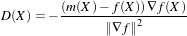 | (3.34) |
However, this equation becomes unstable for small values of the image gradient, resulting in large displacement values. To overcome this problem, Thirion re-normalizes the equation such that:
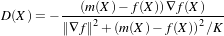 | (3.35) |
Where K is a normalization factor that accounts for the units imbalance between intensities and gradients. This factor is computed as the mean squared value of the pixel spacings. The inclusion of K ensures the force computation is invariant to the pixel scaling of the images.
Starting with an initial deformation field D0(X), the demons algorithm iteratively updates the field using Equation 3.35 such that the field at the N-th iteration is given by:
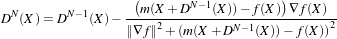 | (3.36) |
Reconstruction of the deformation field is an ill-posed problem where matching the fixed and moving images has many solutions. For example, since each image pixel is free to move independently, it is possible that all pixels of one particular value in m(X) could map to a single image pixel in f(X) of the same value. The resulting deformation field may be unrealistic for real-world applications. An option to solve for the field uniquely is to enforce an elastic-like behavior, smoothing the deformation field with a Gaussian filter between iterations.
In ITK, the demons algorithm is implemented as part of the finite difference solver (FDS) framework and its use is demonstrated in the following example.
The source code for this section can be found in the file
DeformableRegistration2.cxx.
This example demonstrates how to use the “demons” algorithm to deformably register two images. The first step is to include the header files.
Second, we declare the types of the images.
Image file readers are set up in a similar fashion to previous examples. To support the re-mapping of the moving image intensity, we declare an internal image type with a floating point pixel type and cast the input images to the internal image type.
using InternalPixelType = float;
using InternalImageType = itk::Image< InternalPixelType, Dimension >;
using FixedImageCasterType = itk::CastImageFilter< FixedImageType,
InternalImageType >;
using MovingImageCasterType = itk::CastImageFilter< MovingImageType,
InternalImageType >;
FixedImageCasterType::Pointer fixedImageCaster = FixedImageCasterType::New();
MovingImageCasterType::Pointer movingImageCaster
= MovingImageCasterType::New();
fixedImageCaster->SetInput( fixedImageReader->GetOutput() );
movingImageCaster->SetInput( movingImageReader->GetOutput() );
The demons algorithm relies on the assumption that pixels representing the same homologous point on an object have the same intensity on both the fixed and moving images to be registered. In this example, we will preprocess the moving image to match the intensity between the images using the itk::HistogramMatchingImageFilter.
The basic idea is to match the histograms of the two images at a user-specified number of quantile values. For robustness, the histograms are matched so that the background pixels are excluded from both histograms. For MR images, a simple procedure is to exclude all gray values that are smaller than the mean gray value of the image.
For this example, we set the moving image as the source or input image and the fixed image as the reference image.
We then select the number of bins to represent the histograms and the number of points or quantile values where the histogram is to be matched.
Simple background extraction is done by thresholding at the mean intensity.
In the itk::DemonsRegistrationFilter, the deformation field is represented as an image whose pixels are floating point vectors.
using VectorPixelType = itk::Vector< float, Dimension >;
using DisplacementFieldType = itk::Image< VectorPixelType, Dimension >;
using RegistrationFilterType = itk::DemonsRegistrationFilter<
InternalImageType,
InternalImageType,
DisplacementFieldType>;
RegistrationFilterType::Pointer filter = RegistrationFilterType::New();
The input fixed image is simply the output of the fixed image casting filter. The input moving image is the output of the histogram matching filter.
The demons registration filter has two parameters: the number of iterations to be performed and the standard deviation of the Gaussian smoothing kernel to be applied to the deformation field after each iteration.
The registration algorithm is triggered by updating the filter. The filter output is the computed deformation field.
The itk::ResampleImageFilter can be used to warp the moving image with the output deformation field. The default interpolator of the itk::ResampleImageFilter, is used but specification of the output image spacing and origin are required.
using OutputPixelType = unsigned char;
using OutputImageType = itk::Image< OutputPixelType, Dimension >;
using InterpolatorPrecisionType = double;
using WarperType =
itk::ResampleImageFilter< MovingImageType, OutputImageType,
InterpolatorPrecisionType, float >;
WarperType::Pointer warper = WarperType::New();
warper->SetInput( movingImageReader->GetOutput() );
warper->UseReferenceImageOn();
warper->SetReferenceImage( fixedImageReader->GetOutput() );
The ResampleImageFilter requires a transform, so a itk::DisplacementFieldTransform must be constructed then set as the transform of the ResampleImageFilter. The resulting warped or resampled image is written to file as per previous examples.
Let’s execute this example using the rat lung data from the previous example. The associated data files can be found in Examples/Data:
The result of the demons-based deformable registration is presented in Figure 3.48. The checkerboard comparison shows that the algorithm was able to recover the misalignment due to expiration.
It may be also desirable to write the deformation field as an image of vectors. This can be done with the following code.
Note that the file format used for writing the deformation field must be capable of representing multiple components per pixel. This is the case for the MetaImage and VTK file formats for example.
A variant of the force computation is also implemented in which the gradient of the deformed moving image is also involved. This provides a level of symmetry in the force calculation during one iteration of the PDE update. The equation used in this case is
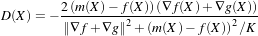 | (3.37) |
The following example illustrates the use of this deformable registration method.
The source code for this section can be found in the file
DeformableRegistration3.cxx.
This example demonstrates how to use a variant of the “demons” algorithm to deformably register two images. This variant uses a different formulation for computing the forces to be applied to the image in order to compute the deformation fields. The variant uses both the gradient of the fixed image and the gradient of the deformed moving image in order to compute the forces. This mechanism for computing the forces introduces a symmetry with respect to the choice of the fixed and moving images. This symmetry only holds during the computation of one iteration of the PDE updates. It is unlikely that total symmetry may be achieved by this mechanism for the entire registration process.
The first step for using this filter is to include the following header files.
Second, we declare the types of the images.
Image file readers are set up in a similar fashion to previous examples. To support the re-mapping of the moving image intensity, we declare an internal image type with a floating point pixel type and cast the input images to the internal image type.
using InternalPixelType = float;
using InternalImageType = itk::Image< InternalPixelType, Dimension >;
using FixedImageCasterType = itk::CastImageFilter< FixedImageType,
InternalImageType >;
using MovingImageCasterType = itk::CastImageFilter< MovingImageType,
InternalImageType >;
FixedImageCasterType::Pointer fixedImageCaster = FixedImageCasterType::New();
MovingImageCasterType::Pointer movingImageCaster
= MovingImageCasterType::New();
fixedImageCaster->SetInput( fixedImageReader->GetOutput() );
movingImageCaster->SetInput( movingImageReader->GetOutput() );
The demons algorithm relies on the assumption that pixels representing the same homologous point on an object have the same intensity on both the fixed and moving images to be registered. In this example, we will preprocess the moving image to match the intensity between the images using the itk::HistogramMatchingImageFilter.
The basic idea is to match the histograms of the two images at a user-specified number of quantile values. For robustness, the histograms are matched so that the background pixels are excluded from both histograms. For MR images, a simple procedure is to exclude all gray values that are smaller than the mean gray value of the image.
For this example, we set the moving image as the source or input image and the fixed image as the reference image.
We then select the number of bins to represent the histograms and the number of points or quantile values where the histogram is to be matched.
Simple background extraction is done by thresholding at the mean intensity.
In the itk::SymmetricForcesDemonsRegistrationFilter, the deformation field is represented as an image whose pixels are floating point vectors.
using VectorPixelType = itk::Vector< float, Dimension >;
using DisplacementFieldType = itk::Image< VectorPixelType, Dimension >;
using RegistrationFilterType = itk::SymmetricForcesDemonsRegistrationFilter<
InternalImageType,
InternalImageType,
DisplacementFieldType>;
RegistrationFilterType::Pointer filter = RegistrationFilterType::New();
The input fixed image is simply the output of the fixed image casting filter. The input moving image is the output of the histogram matching filter.
The demons registration filter has two parameters: the number of iterations to be performed and the standard deviation of the Gaussian smoothing kernel to be applied to the deformation field after each iteration.
The registration algorithm is triggered by updating the filter. The filter output is the computed deformation field.
The itk::WarpImageFilter can be used to warp the moving image with the output deformation field. Like the itk::ResampleImageFilter, the WarpImageFilter requires the specification of the input image to be resampled, an input image interpolator, and the output image spacing and origin.
using WarperType = itk::WarpImageFilter<
MovingImageType,
MovingImageType,
DisplacementFieldType >;
using InterpolatorType = itk::LinearInterpolateImageFunction<
MovingImageType,
double >;
WarperType::Pointer warper = WarperType::New();
InterpolatorType::Pointer interpolator = InterpolatorType::New();
FixedImageType::Pointer fixedImage = fixedImageReader->GetOutput();
warper->SetInput( movingImageReader->GetOutput() );
warper->SetInterpolator( interpolator );
warper->SetOutputSpacing( fixedImage->GetSpacing() );
warper->SetOutputOrigin( fixedImage->GetOrigin() );
warper->SetOutputDirection( fixedImage->GetDirection() );
Unlike the ResampleImageFilter, the WarpImageFilter warps or transforms the input image with respect to the deformation field represented by an image of vectors. The resulting warped or resampled image is written to file as per previous examples.
Let’s execute this example using the rat lung data from the previous example. The associated data files can be found in Examples/Data:
The result of the demons-based deformable registration is presented in Figure 3.49. The checkerboard comparison shows that the algorithm was able to recover the misalignment due to expiration.
It may be also desirable to write the deformation field as an image of vectors. This can be done with the following code.
Note that the file format used for writing the deformation field must be capable of representing multiple components per pixel. This is the case for the MetaImage and VTK file formats for example.
Vector deformation fields may be visualized using ParaView. ParaView [25] is an open-source, multi-platform visualization application and uses the Visualization Toolkit as the data processing and rendering engine and has a user interface written using a unique blend of Tcl/Tk and C++. You may download it from http://paraview.org.
Let us visualize the deformation field obtained from Demons Registration algorithm generated from ITK/Examples/RegistrationITKv4/DeformableRegistration2.cxx.
Load the Deformation field in Paraview. (The deformation field must be capable of handling vector data, such as MetaImages). Paraview shows a color map of the magnitudes of the deformation fields as shown in 3.50.
Covert the deformation field to 3D vector data using a Calculator. The Calculator may be found in the Filter pull down menu. A screenshot of the calculator tab is shown in Figure 3.51. Although the deformation field is a 2D vector, we will generate a 3D vector with the third component set to 0 since Paraview generates glyphs only for 3D vectors. You may now apply a glyph of arrows to the resulting 3D vector field by using Glyph on the menu bar. The glyphs obtained will be very dense since a glyph is generated for each point in the data set. To better visualize the deformation field, you may adopt one of the following approaches.
Reduce the number of glyphs by reducing the number in Max. Number of Glyphs to a reasonable amount. This uniformly downsamples the number of glyphs. Alternatively, you may apply a Threshold filter to the Magnitude of the vector dataset and then glyph the vector data that lie above the threshold. This eliminates the smaller deformation fields that clutter the display. You may now reduce the number of glyphs to a reasonable value.
Figure 3.52 shows the vector field visualized using Paraview by thresholding the vector magnitudes by 2.1 and restricting the number of glyphs to 100.
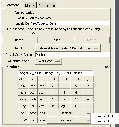
Let us create a 3D deformation field. We will use Thin Plate Splines to warp a 3D dataset and create a deformation field. We will pick a set of point landmarks and translate them to provide a specification of correspondences at point landmarks. Note that the landmarks have been picked randomly for purposes of illustration and are not intended to portray a true deformation. The landmarks may be used to produce a deformation field in several ways. Most techniques minimize some regularizing functional representing the irregularity of the deformation field, which is usually some function of the spatial derivatives of the field. Here will we use thin plate splines. Thin plate splines minimize the regularizing functional
![∫∫ 2 2 2
I[f (x,y)]= (fxx+ 2fxy+ fyy)dxdy](ITKSoftwareGuide-Book2300x.png) | (3.38) |
where the subscripts denote partial derivatives of f.
We may now proceed as before to visualize the deformation field using Paraview as shown in Figure 3.53.
Let us register the deformed volumes generated by Thin plate warping in the previous example using DeformableRegistration4.cxx. Since ITK is in general N-dimensional, the only change in the example is to replace the ImageDimension by 3.
The registration method uses B-splines and an LBFGS optimizer. The trace in Table. 3.17 prints the trace of the optimizer through the search space.
| Iteration | Function value | ∥G∥ | Step length |
| 1 | 156.981 | 14.911 | 0.202 |
| 2 | 68.956 | 11.774 | 1.500 |
| 3 | 38.146 | 4.802 | 1.500 |
| 4 | 26.690 | 2.515 | 1.500 |
| 5 | 23.295 | 1.106 | 1.500 |
| 6 | 21.454 | 1.032 | 1.500 |
| 7 | 20.322 | 1.557 | 1.500 |
| 8 | 19.751 | 0.594 | 1.500 |
Here ∥G∥ is the norm of the gradient at the current estimate of the minimum, x. “Function Value” is the current value of the function, f(x).
The resulting deformation field that maps the moving to the fixed image is shown in 3.54. A difference image of two slices before and after registration is shown in 3.55. As can be seen from the figures, the deformation field is in close agreement to the one generated from the Thin plate spline warping.
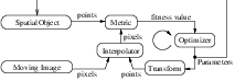
Figure 3.56: The basic components of model based
registration are an image, a spatial object, a transform, a
metric, an interpolator and an optimizer.
This section introduces the concept of registering a geometrical model with an image. We refer to this concept as model based registration but this may not be the most widespread terminology. In this approach, a geometrical model is built first and a number of parameters are identified in the model. Variations of these parameters make it possible to adapt the model to the morphology of a particular patient. The task of registration is then to find the optimal combination of model parameters that will make this model a good representation of the anatomical structures contained in an image.
For example, let’s say that in the axial view of a brain image we can roughly approximate the skull with an ellipse. The ellipse becomes our simplified geometrical model, and registration is the task of finding the best center for the ellipse, the measures of its axis lengths and its orientation in the plane. This is illustrated in Figure 3.57. If we compare this approach with the image-to-image registration problem, we can see that the main difference here is that in addition to mapping the spatial position of the model, we can also customize internal parameters that change its shape.
Figure 3.56 illustrates the major components of the registration framework in ITK when a model-based registration problem is configured. The basic input data for the registration is provided by pixel data in an itk::Image and by geometrical data stored in a itk::SpatialObject. A metric has to be defined in order to evaluate the fitness between the model and the image. This fitness value can be improved by introducing variations in the spatial positioning of the SpatialObject and/or by changing its internal parameters. The search space for the optimizer is now the composition of the transform parameter and the shape internal parameters.
This same approach can be considered a segmentation technique, since once the model has been optimally superimposed on the image we could label pixels according to their associations with specific parts of the model. The applications of model to image registration/segmentation are endless. The main advantage of this approach is probably that, as opposed to image-to-image registration, it actually provides Insight into the anatomical structure contained in the image. The adapted model becomes a condensed representation of the essential elements of the anatomical structure.
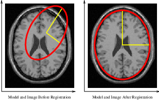
ITK provides a hierarchy of classes intended to support the construction of shape models. This hierarchy has the SpatialObject as its base class. A number of basic functionalities are defined at this level, including the capacity to evaluate whether a given point is inside or outside of the model, form complex shapes by creating hierarchical conglomerates of basic shapes, and support basic spatial parameterizations like scale, orientation and position.
The following sections present examples of the typical uses of these powerful elements of the toolkit.
The source code for this section can be found in the file
ModelToImageRegistration1.cxx.
This example illustrates the use of the itk::SpatialObject as a component of the registration framework in order to perform model based registration. The current example creates a geometrical model composed of several ellipses. Then, it uses the model to produce a synthetic binary image of the ellipses. Next, it introduces perturbations on the position and shape of the model, and finally it uses the perturbed version as the input to a registration problem. A metric is defined to evaluate the fitness between the geometric model and the image.
Let’s look first at the classes required to support SpatialObject. In this example we use the itk::EllipseSpatialObject as the basic shape components and we use the itk::GroupSpatialObject to group them together as a representation of a more complex shape. Their respective headers are included below.
In order to generate the initial synthetic image of the ellipses, we use the itk::SpatialObjectToImageFilter that tests—for every pixel in the image—whether the pixel (and hence the spatial object) is inside or outside the geometric model.
A metric is defined to evaluate the fitness between the SpatialObject and the Image. The base class for this type of metric is the itk::ImageToSpatialObjectMetric, whose header is included below.
As in previous registration problems, we have to evaluate the image intensity in non-grid positions. The itk::LinearInterpolateImageFunction is used here for this purpose.
The SpatialObject is mapped from its own space into the image space by using a itk::Transform. In this example, we use the itk::Euler2DTransform.
Registration is fundamentally an optimization problem. Here we include the optimizer used to search the parameter space and identify the best transformation that will map the shape model on top of the image. The optimizer used in this example is the itk::OnePlusOneEvolutionaryOptimizer that implements an evolutionary algorithm.
As in previous registration examples, it is important to track the evolution of the optimizer as it progresses through the parameter space. This is done by using the Command/Observer paradigm. The following lines of code implement the itk::Command observer that monitors the progress of the registration. The code is quite similar to what we have used in previous registration examples.
#include "itkCommand.h"
template < class TOptimizer >
class IterationCallback : public itk::Command
{
public:
using Self = IterationCallback;
using Superclass = itk::Command;
using Pointer = itk::SmartPointer<Self>;
using ConstPointer = itk::SmartPointer<const Self>;
itkTypeMacro( IterationCallback, Superclass );
itkNewMacro( Self );
/⋆⋆ Type defining the optimizer. ⋆/
using OptimizerType = TOptimizer;
/⋆⋆ Method to specify the optimizer. ⋆/
void SetOptimizer( OptimizerType ⋆ optimizer )
{
m_Optimizer = optimizer;
m_Optimizer->AddObserver( itk::IterationEvent(), this );
}
/⋆⋆ Execute method will print data at each iteration ⋆/
void Execute(itk::Object ⋆caller,
const itk::EventObject & event) override
{
Execute( (const itk::Object ⋆)caller, event);
}
void Execute(const itk::Object ⋆,
const itk::EventObject & event) override
{
if( typeid( event ) == typeid( itk::StartEvent ) )
{
std::cout << std::endl << "Position Value";
std::cout << std::endl << std::endl;
}
else if( typeid( event ) == typeid( itk::IterationEvent ) )
{
std::cout << m_Optimizer->GetCurrentIteration() << " ";
std::cout << m_Optimizer->GetValue() << " ";
std::cout << m_Optimizer->GetCurrentPosition() << std::endl;
}
else if( typeid( event ) == typeid( itk::EndEvent ) )
{
std::cout << std::endl << std::endl;
std::cout << "After " << m_Optimizer->GetCurrentIteration();
std::cout << " iterations " << std::endl;
std::cout << "Solution is = " << m_Optimizer->GetCurrentPosition();
std::cout << std::endl;
}
}
This command will be invoked at every iteration of the optimizer and will print out the current combination of transform parameters.
Consider now the most critical component of this new registration approach: the metric. This component evaluates the match between the SpatialObject and the Image. The smoothness and regularity of the metric determine the difficulty of the task assigned to the optimizer. In this case, we use a very robust optimizer that should be able to find its way even in the most discontinuous cost functions. The metric to be implemented should derive from the ImageToSpatialObjectMetric class.
The following code implements a simple metric that computes the sum of the pixels that are inside the spatial object. In fact, the metric maximum is obtained when the model and the image are aligned. The metric is templated over the type of the SpatialObject and the type of the Image.
The fundamental operation of the metric is its GetValue() method. It is in this method that the fitness value is computed. In our current example, the fitness is computed over the points of the SpatialObject. For each point, its coordinates are mapped through the transform into image space. The resulting point is used to evaluate the image and the resulting value is accumulated in a sum. Since we are not allowing scale changes, the optimal value of the sum will result when all the SpatialObject points are mapped on the white regions of the image. Note that the argument for the GetValue() method is the array of parameters of the transform.
MeasureType GetValue( const ParametersType & parameters ) const override
{
double value;
this->m_Transform->SetParameters( parameters );
value = 0;
for(auto it = m_PointList.begin(); it != m_PointList.end(); ++it)
{
PointType transformedPoint = this->m_Transform->TransformPoint(⋆it);
if( this->m_Interpolator->IsInsideBuffer( transformedPoint ) )
{
value += this->m_Interpolator->Evaluate( transformedPoint );
}
}
return value;
}
Having defined all the registration components we are ready to put the pieces together and implement the registration process.
First we instantiate the GroupSpatialObject and EllipseSpatialObject. These two objects are parameterized by the dimension of the space. In our current example a 2D instantiation is created.
The image is instantiated in the following lines using the pixel type and the space dimension. This image uses a float pixel type since we plan to blur it in order to increase the capture radius of the optimizer. Images of real pixel type behave better under blurring than those of integer pixel type.
Here is where the fun begins! In the following lines we create the EllipseSpatialObjects using their New() methods, and assigning the results to SmartPointers. These lines will create three ellipses.
Every class deriving from SpatialObject has particular parameters enabling the user to tailor its shape. In the case of the EllipseSpatialObject, SetRadius() is used to define the ellipse size. An additional SetRadius(Array) method allows the user to define the ellipse axes independently.
The ellipses are created centered in space by default. We use the following lines of code to arrange the ellipses in a triangle. The spatial transform intrinsically associated with the object is accessed by the GetTransform() method. This transform can define a translation in space with the SetOffset() method. We take advantage of this feature to place the ellipses at particular points in space.
EllipseType::TransformType::OffsetType offset;
offset[ 0 ] = 100.0;
offset[ 1 ] = 40.0;
ellipse1->GetModifiableObjectToParentTransform()->SetOffset(offset);
ellipse1->Update();
offset[ 0 ] = 40.0;
offset[ 1 ] = 150.0;
ellipse2->GetModifiableObjectToParentTransform()->SetOffset(offset);
ellipse2->Update();
offset[ 0 ] = 150.0;
offset[ 1 ] = 150.0;
ellipse3->GetModifiableObjectToParentTransform()->SetOffset(offset);
ellipse3->Update();
Note that after a change has been made in the transform, the SpatialObject invokes the method ComputeGlobalTransform() in order to update its global transform. The reason for doing this is that SpatialObjects can be arranged in hierarchies. It is then possible to change the position of a set of spatial objects by moving the parent of the group.
Now we add the three EllipseSpatialObjects to a GroupSpatialObject that will be subsequently passed on to the registration method. The GroupSpatialObject facilitates the management of the three ellipses as a higher level structure representing a complex shape. Groups can be nested any number of levels in order to represent shapes with higher detail.
Having the geometric model ready, we proceed to generate the binary image representing the imprint of the space occupied by the ellipses. The SpatialObjectToImageFilter is used to that end. Note that this filter is instantiated over the spatial object used and the image type to be generated.
With the defined type, we construct a filter using the New() method. The newly created filter is assigned to a SmartPointer.
The GroupSpatialObject is passed as input to the filter.
The itk::SpatialObjectToImageFilter acts as a resampling filter. Therefore it requires the user to define the size of the desired output image. This is specified with the SetSize() method.
Finally we trigger the execution of the filter by calling the Update() method.
In order to obtain a smoother metric, we blur the image using a itk::DiscreteGaussianImageFilter. This extends the capture radius of the metric and produce a more continuous cost function to optimize. The following lines instantiate the Gaussian filter and create one object of this type using the New() method.
The output of the SpatialObjectToImageFilter is connected as input to the DiscreteGaussianImageFilter.
The variance of the filter is defined as a large value in order to increase the capture radius. Finally the execution of the filter is triggered using the Update() method.
Below we instantiate the type of the itk::ImageToSpatialObjectRegistrationMethod method and instantiate a registration object with the New() method. Note that the registration type is templated over the Image and the SpatialObject types. The spatial object in this case is the group of spatial objects.
Now we instantiate the metric that is templated over the image type and the spatial object type. As usual, the New() method is used to create an object.
An interpolator will be needed to evaluate the image at non-grid positions. Here we instantiate a linear interpolator type.
The following lines instantiate the evolutionary optimizer.
Next, we instantiate the transform class. In this case we use the Euler2DTransform that implements a rigid transform in 2D space.
Evolutionary algorithms are based on testing random variations of parameters. In order to support the computation of random values, ITK provides a family of random number generators. In this example, we use the itk::NormalVariateGenerator which generates values with a normal distribution.
The random number generator must be initialized with a seed.
The OnePlusOneEvolutionaryOptimizer is initialized by specifying the random number generator, the number of samples for the initial population and the maximum number of iterations.
As in previous registration examples, we take care to normalize the dynamic range of the different transform parameters. In particular, the we must compensate for the ranges of the angle and translations of the Euler2DTransform. In order to achieve this goal, we provide an array of scales to the optimizer.
Here we instantiate the Command object that will act as an observer of the registration method and print out parameters at each iteration. Earlier, we defined this command as a class templated over the optimizer type. Once it is created with the New() method, we connect the optimizer to the command.
All the components are plugged into the ImageToSpatialObjectRegistrationMethod object. The typical Set() methods are used here. Note the use of the SetMovingSpatialObject() method for connecting the spatial object. We provide the blurred version of the original synthetic binary image as the input image.
The initial set of transform parameters is passed to the registration method using the SetInitialTransformParameters() method. Note that since our original model is already registered with the synthetic image, we introduce an artificial mis-registration in order to initialize the optimization at some point away from the optimal value.
Due to the character of the metric used to evaluate the fitness between the spatial object and the image, we must tell the optimizer that we are interested in finding the maximum value of the metric. Some metrics associate low numeric values with good matching, while others associate high numeric values with good matching. The MaximizeOn() and MaximizeOff() methods allow the user to deal with both types of metrics.
Finally, we trigger the execution of the registration process with the Update() method. We place this call in a try/catch block in case any exception is thrown during the process.
The set of transform parameters resulting from the registration can be recovered with the GetLastTransformParameters() method. This method returns the array of transform parameters that should be interpreted according to the implementation of each transform. In our current example, the Euler2DTransform has three parameters: the rotation angle, the translation in x and the translation in y.
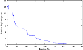
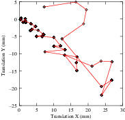
The results are presented in Figure 3.58. The left side shows the evolution of the angle parameter as a function of iteration numbers, while the right side shows the (x,y) translation.
PointSet-to-PointSet registration is a common problem in medical image analysis. It usually arises in cases where landmarks are extracted from images and are used for establishing the spatial correspondence between the images. This type of registration can be considered to be the simplest case of feature-based registration. In general terms, feature-based registration is more efficient than the intensity based method that we have presented so far. However, feature-base registration brings the new problem of identifying and extracting the features from the images, which is not a minor challenge.
The two most common scenarios in PointSet to PointSet registration are
The first case can be solved with a closed form solution when we are dealing with a Rigid or an Affine Transform [26]. This is done in ITK with the class itk::LandmarkBasedTransformInitializer. If we are interested in a deformable Transformation then the problem can be solved with the itk::KernelTransform family of classes, which includes Thin Plate Splines among others [51]. In both circumstances, the availability o f correspondences between the points make possible to apply a straight forward solution to the problem.
The classical algorithm for performing PointSet to PointSet registration is the Iterative Closest Point (ICP) algorithm. The following examples illustrate how this can be used in ITK.
The source code for this section can be found in the file
IterativeClosestPoint1.cxx.
This example illustrates how to perform Iterative Closest Point (ICP) registration in ITK. The main class featured in this section is the itk::EuclideanDistancePointMetric.
The first step is to include the relevant headers.
Next, define the necessary types for the fixed and moving pointsets and point containers.
constexpr unsigned int Dimension = 2;
using PointSetType = itk::PointSet< float, Dimension >;
PointSetType::Pointer fixedPointSet = PointSetType::New();
PointSetType::Pointer movingPointSet = PointSetType::New();
using PointType = PointSetType::PointType;
using PointsContainer = PointSetType::PointsContainer;
PointsContainer::Pointer fixedPointContainer = PointsContainer::New();
PointsContainer::Pointer movingPointContainer = PointsContainer::New();
PointType fixedPoint;
PointType movingPoint;
After the points are read in from files, set up the metric type.
Now, setup the transform, optimizers, and registration method using the point set types defined earlier.
using TransformType = itk::TranslationTransform< double, Dimension >;
TransformType::Pointer transform = TransformType::New();
// Optimizer Type
using OptimizerType = itk::LevenbergMarquardtOptimizer;
OptimizerType::Pointer optimizer = OptimizerType::New();
optimizer->SetUseCostFunctionGradient(false);
// Registration Method
using RegistrationType = itk::PointSetToPointSetRegistrationMethod<
PointSetType, PointSetType >;
RegistrationType::Pointer registration = RegistrationType::New();
// Scale the translation components of the Transform in the Optimizer
OptimizerType::ScalesType scales( transform->GetNumberOfParameters() );
scales.Fill( 0.01 );
Next we setup the convergence criteria, and other properties required by the optimizer.
unsigned long numberOfIterations = 100;
double gradientTolerance = 1e-5; // convergence criterion
double valueTolerance = 1e-5; // convergence criterion
double epsilonFunction = 1e-6; // convergence criterion
optimizer->SetScales( scales );
optimizer->SetNumberOfIterations( numberOfIterations );
optimizer->SetValueTolerance( valueTolerance );
optimizer->SetGradientTolerance( gradientTolerance );
optimizer->SetEpsilonFunction( epsilonFunction );
In this case we start from an identity transform, but in reality the user will usually be able to provide a better guess than this.
Finally, connect all the components required for the registration, and an observer.
registration->SetMetric( metric );
registration->SetOptimizer( optimizer );
registration->SetTransform( transform );
registration->SetFixedPointSet( fixedPointSet );
registration->SetMovingPointSet( movingPointSet );
// Connect an observer
CommandIterationUpdate::Pointer observer = CommandIterationUpdate::New();
optimizer->AddObserver( itk::IterationEvent(), observer );
The source code for this section can be found in the file
IterativeClosestPoint2.cxx.
This example illustrates how to perform Iterative Closest Point (ICP) registration in ITK using sets of 3D points.
The first step is to include the relevant headers.
First, define the necessary types for the moving and fixed point sets.
using PointSetType = itk::PointSet< float, Dimension >;
PointSetType::Pointer fixedPointSet = PointSetType::New();
PointSetType::Pointer movingPointSet = PointSetType::New();
using PointType = PointSetType::PointType;
using PointsContainer = PointSetType::PointsContainer;
PointsContainer::Pointer fixedPointContainer = PointsContainer::New();
PointsContainer::Pointer movingPointContainer = PointsContainer::New();
PointType fixedPoint;
PointType movingPoint;
After the points are read in from files, setup the metric to be used later by the registration.
Next, setup the tranform, optimizers, and registration.
using TransformType = itk::Euler3DTransform< double >;
TransformType::Pointer transform = TransformType::New();
// Optimizer Type
using OptimizerType = itk::LevenbergMarquardtOptimizer;
OptimizerType::Pointer optimizer = OptimizerType::New();
optimizer->SetUseCostFunctionGradient(false);
// Registration Method
using RegistrationType = itk::PointSetToPointSetRegistrationMethod<
PointSetType, PointSetType >;
RegistrationType::Pointer registration = RegistrationType::New();
Scale the translation components of the Transform in the Optimizer
Next, set the scales and ranges for translations and rotations in the transform. Also, set the convergence criteria and number of iterations to be used by the optimizer.
constexpr double translationScale = 1000.0; // dynamic range of translations
constexpr double rotationScale = 1.0; // dynamic range of rotations
scales[0] = 1.0 / rotationScale;
scales[1] = 1.0 / rotationScale;
scales[2] = 1.0 / rotationScale;
scales[3] = 1.0 / translationScale;
scales[4] = 1.0 / translationScale;
scales[5] = 1.0 / translationScale;
unsigned long numberOfIterations = 2000;
double gradientTolerance = 1e-4; // convergence criterion
double valueTolerance = 1e-4; // convergence criterion
double epsilonFunction = 1e-5; // convergence criterion
optimizer->SetScales( scales );
optimizer->SetNumberOfIterations( numberOfIterations );
optimizer->SetValueTolerance( valueTolerance );
optimizer->SetGradientTolerance( gradientTolerance );
optimizer->SetEpsilonFunction( epsilonFunction );
Here we start with an identity transform, although the user will usually be able to provide a better guess than this.
Connect all the components required for the registration.
The source code for this section can be found in the file
IterativeClosestPoint3.cxx.
This example illustrates how to perform Iterative Closest Point (ICP) registration in ITK using a DistanceMap in order to increase the performance. There is of course a trade-off between the time needed for computing the DistanceMap and the time saved by its repeated use during the iterative computation of the point-to-point distances. It is then necessary in practice to ponder both factors.
itk::EuclideanDistancePointMetric.
The first step is to include the relevant headers.
#include "itkTranslationTransform.h"
#include "itkEuclideanDistancePointMetric.h"
#include "itkLevenbergMarquardtOptimizer.h"
#include "itkPointSetToPointSetRegistrationMethod.h"
#include "itkDanielssonDistanceMapImageFilter.h"
#include "itkPointSetToImageFilter.h"
#include <iostream>
#include <fstream>
Next, define the necessary types for the fixed and moving point sets.
using PointSetType = itk::PointSet< float, Dimension >;
PointSetType::Pointer fixedPointSet = PointSetType::New();
PointSetType::Pointer movingPointSet = PointSetType::New();
using PointType = PointSetType::PointType;
using PointsContainer = PointSetType::PointsContainer;
PointsContainer::Pointer fixedPointContainer = PointsContainer::New();
PointsContainer::Pointer movingPointContainer = PointsContainer::New();
PointType fixedPoint;
PointType movingPoint;
Setup the metric, transform, optimizers and registration in a manner similar to the previous two examples.
In the preparation of the distance map, we first need to map the fixed points into a binary image.
using BinaryImageType = itk::Image< unsigned char, Dimension >;
using PointsToImageFilterType = itk::PointSetToImageFilter<
PointSetType,
BinaryImageType>;
PointsToImageFilterType::Pointer
pointsToImageFilter = PointsToImageFilterType::New();
pointsToImageFilter->SetInput( fixedPointSet );
BinaryImageType::SpacingType spacing;
spacing.Fill( 1.0 );
BinaryImageType::PointType origin;
origin.Fill( 0.0 );
Continue to prepare the distance map, in order to accelerate the distance computations.
pointsToImageFilter->SetSpacing( spacing );
pointsToImageFilter->SetOrigin( origin );
pointsToImageFilter->Update();
BinaryImageType::Pointer binaryImage = pointsToImageFilter->GetOutput();
using DistanceImageType = itk::Image< unsigned short, Dimension >;
using DistanceFilterType = itk::DanielssonDistanceMapImageFilter<
BinaryImageType, DistanceImageType>;
DistanceFilterType::Pointer distanceFilter = DistanceFilterType::New();
distanceFilter->SetInput( binaryImage );
distanceFilter->Update();
metric->SetDistanceMap( distanceFilter->GetOutput() );
So you read the previous sections, you wrote the code, it compiles and links fine, but when you run it the registration results are not what you were expecting. In that case, this section is for you. This is a compilation of the most common problems that users face when performing image registration. It provides explanations on the potential sources of the problems, and advice on how to deal with those problems.
Most of the material in this section has been taken from frequently asked questions of the ITK users list.
http://public.kitware.com/pipermail/insight-users/2007-March/021442.html
This is a common error message in image registration.
It means that at the current iteration of the optimization, the two images as so off-registration that their spatial overlap is not large enough for bringing them back into registration.
The common causes of this problem are:
Increasing the step length makes your program faster, but it also makes it more unstable.
In typical medical datasets such as CT and MR, translations are measured in millimeters, and therefore are in the range of -100:100, while rotations are measured in radians, and therefore they tend to be in the range of -1:1.
A rotation of 3 radians is catastrophic, while a translation of 3 millimeters is rather inoffensive. That difference in scale is the one that must be accounted for.
http://public.kitware.com/pipermail/insight-users/2007-March/021435.html
Here is some advice on how to fine tune the parameters of the registration process.
1) Set Maximum step length to 0.1 and do not change it until all other parameters are stable.
2) Set Minimum step length to 0.001 and do not change it.
You could interpret these two parameters as if their units were radians. So, 0.1 radian = 5.7 degrees.
3) Number of histogram bins:
First plot the histogram of your image using the example program in
Insight/Examples/Statistics/ImageHistogram2.cxx
In that program use first a large number of bins (for example 2000) and identify the different populations of intensity level and to what anatomical structures they correspond.
Once you identify the anatomical structures in the histogram, then rerun that same program with less and less number of bins, until you reach the minimun number of bins for which all the tissues that are important for your application, are still distinctly differentiated in the histogram. At that point, take that number of bins and us it for your Mutual Information metric.
4) Number of Samples: The trade-off with the number of samples is the following:
a) computation time of registration is linearly proportional to the number of samples b) the samples must be enough to significantly populate the joint histogram. c) Once the histogram is populated, there is not much use in adding more samples. Therefore do the following:
Plot the joint histogram of both images, using the number of bins that you selected in item (3). You can do this by modifying the code of the example:
Insight/Examples/Statistics/ ImageMutualInformation1.cxx you have to change the code to print out the values of the bins. Then use a plotting program such as gnuplot, or Matlab, or even Excel and look at the distribution. The number of samples to take must be enough for producing the same ”appearance” of the joint histogram. As an arbitrary rule of thumb you may want to start using a high number of samples (80% - 100%). And do not change it until you have mastered the other parameters of the registration. Once you get your registration to converge you can revisit the number of samples and reduce it in order to make the registration run faster. You can simply reduce it until you find that the registration becomes unstable. That’s your critical bound for the minimum number of samples. Take that number and multiply it by the magic number 1.5, to send it back to a stable region, or if your application is really critical, then use an even higher magic number x2.0.
This is just engineering: you figure out what is the minimal size of a piece of steel that will support a bridge, and then you enlarge it to keep it away from the critical value.
5) The MOST critical values of the registration process are the scaling parameters that define the proportions between the parameters of the transform. In your case, for an Affine Transform in 2D, you have 6 parameters. The first four are the ones of the Matrix, and the last two are the translation. The rotation matrix value must be in the ranges of radians which is typically [ -1 to 1 ], while the translation values are in the ranges of millimeters (your image size units). You want to start by setting the scaling of the matrix parameters to 1.0, and the scaling of the Translation parameters to the holy esoteric values:
1.0 / ( 10.0 * pixelspacing[0] * imagesize[0] ) 1.0 / ( 10.0 * pixelspacing[1] * imagesize[1] )
This is telling the optimizer that you consider that rotating the image by 57 degrees is as ”significant” as translating the image by half its physical extent.
Note that esoteric value has included the arbitrary number 10.0 in the denominator, for no other reason that we have been lucky when using that factor. This of course is just a superstition, so you should feel free to experiment with different values of this number.
Just keep in mind that what the optimizer will do is to “jump” in a parametric space of 6 dimensions, and that the component of the jump on every dimension will be proportional to 1/scaling factor * OptimizerStepLength. Since you set the optimizer Step Length to 0.1, the optimizer will start by exploring the rotations at jumps of about 5 degrees, which is a conservative rotation for most medical applications.
If you have reasons to think that your rotations are larger or smaller, then you should modify the scaling factor of the matrix parameters accordingly.
In the same way, if you think that 1/10 of the image size is too large as the first step for exploring the translations, then you should modify the scaling of translation parameters accordingly.
In order to drive all these you need to analyze the feedback that the observer is providing you. For example, plot the metric values, and plot the translation coordinates so that you can get a feeling of how the registration is behaving.
Note also that image registration is not a science. It is a pure engineerig practice, and therefore, there are no correct answers, nor “truths” to be found. It is all about how much quality you want, and how must computation time, and development time you are willing to pay for that quality. The “satisfying” answer for your specific application must be found by exploring the trade-offs between the different parameters that regulate the image registration process.
If you are proficient in VTK you may want to consider attaching some visualization to the Event observer, so that you can have a visual feedback on the progress of the registration. This is a lot more productive than trying to interpret the values printed out on the console by the observer.